Core Simulation

The main simulation functions used for adding, running, and visualizing ODEs

Preliminaries

pyndamics3 version 0.0.32

patch

 patch (f)

Decorator: add f to the first parameter’s class (based on f’s type annotations)

source

patch_to

 patch_to (cls, as_prop=False)

Decorator: add f to cls

source

copy_func

 copy_func (f)

Copy a non-builtin function (NB copy.copy does not work for this)

source

RedirectStdStreams

 RedirectStdStreams (stdout=None, stderr=None)

Initialize self. See help(type(self)) for accurate signature.

source

InterpFunction

 InterpFunction (x, y, name)

Initialize self. See help(type(self)) for accurate signature.

source

array_wrap

 array_wrap (_f)

source

from_values

 from_values (var, *args)

Supporting functions for solving ODE and MAPS

source

simfunc

 simfunc (_vec, t, _sim)

source

rk45

 rk45 (function, y0, t_mat, _self, *args, **kwargs)

source

rkwrapper

 rkwrapper (function, _self)

source

rk4

 rk4 (function, y0, t_mat, *args, **kwargs)

source

rk2

 rk2 (function, y0, t_mat, *args, **kwargs)

source

euler

 euler (function, y0, t_mat, *args, **kwargs)

source

mapsolve

 mapsolve (function, y0, t_mat, *args)

source

vector_field

 vector_field (sim, rescale=False, **kwargs)

source

phase_plot

 phase_plot (sim, x, y, z=None, **kwargs)

Make a Phase Plot of two or three variables.

	Type	Default	Details
sim	Simulation		This is a simulation object.
x	str		Name of the variable to plot on the x-axis
y	str		Name of the variable to plot on the y-axis
z	NoneType	None	Name of the variable to plot on the (optional) z-axis
kwargs
Returns

source

Component

 Component (diffstr, initial_value=0, min=None, max=None, plot=False,
            save=None)

Initialize self. See help(type(self)) for accurate signature.

Examples of Components

The `Simulation` class is the primary one to use

source

Simulation

 Simulation (method='odeint', verbose=False, plot_style='.-')

Initialize self. See help(type(self)) for accurate signature.

An alternate way of specifying the equations - stocks, inflows and outflows

@patch
def inflow(self:Simulation,cname,s):

    c=[x for x in self.components if x.name==cname]

    if not c:
        raise ValueError('No component named "%s"' % cname)

    c[0].inflow(s)

@patch
def outflow(self:Simulation,cname,s):

    c=[x for x in self.components if x.name==cname]

    if not c:
        raise ValueError('No component named "%s"' % cname)

    c[0].outflow(s)

@patch
def stock(self:Simulation,name,initial_value=0,
                min=None,max=None,
                plot=False,save=None):

    c=Component(name+"'=",initial_value,min,max,plot,save)
    self.components.append(c)
    return c

sim=Simulation()
sim.add("y'=a - b*y",100)
sim.params(a=10,b=2)
print(sim.equations())

y'=a - b*y
a=10
b=2

#sim.add("y'=a - b*y",100)

sim=Simulation()
sim.stock("y",100)
sim.inflow('y','a')
sim.outflow('y','b*y')
sim.params(a=10,b=2)
print(sim.equations())

y'=+a-(b*y)
a=10
b=2

Some useful functions

source

mse_from_sim

 mse_from_sim (params, extra)

source

model

 model (params, xd, sim, varname, parameters)

source

repeat

 repeat (S_orig, t_min, t_max, **kwargs)

This is my solution to an age-old problem of storing data in loops

source

Storage

 Storage (save_every=1)

Initialize self. See help(type(self)) for accurate signature.

y=1
x=0
dx=0.01
a=0.1

S=Storage()  # this object will store data
S+=x,y   # adds this to the store, one data point at a time
while x<=10:
    dy=a*y*(50-y)*dx
    y+=dy
    x+=dx
    
    S+=x,y  # adds this to the store, one data point at a time
    
x,y=S.arrays()  # returns an array representation of all those data points
plot(x,y)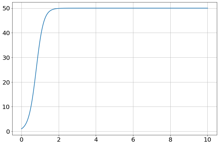

x,y

(array([0.000e+00, 1.000e-02, 2.000e-02, ..., 9.990e+00, 1.000e+01,
        1.001e+01]),
 array([ 1.       ,  1.049    ,  1.1003496, ..., 50.       , 50.       ,
        50.       ]))

source

pso_fit_sim

 pso_fit_sim (varname, xd, yd, sim, parameters, n_particles=30,
              n_iterations=-1, progress_interval=100, plot=False)

source

swarm

 swarm (parameters, fitness, number_of_particles=30, extra=None)

Initialize self. See help(type(self)) for accurate signature.

source

particle

 particle (parameters, fitness_function, extra=None)

Initialize self. See help(type(self)) for accurate signature.

Stochastic Sims

source

Stochastic_Component

 Stochastic_Component (name, initial_value=0, assignment_str=None,
                       min=None, max=None, plot=False, save=None)

Initialize self. See help(type(self)) for accurate signature.

source

Stochastic_Simulation

 Stochastic_Simulation ()

Initialize self. See help(type(self)) for accurate signature.

source

Struct

β=0.2
γ=0.1
So=990
Io=10

dynamic_sim=sim=Simulation()
sim.add("N=S+I+R")
sim.add("S'=-β*S*I/N",So)
sim.add("I'=+β*S*I/N-γ*I",Io)
sim.add("R'=+γ*I",0)
sim.params(β=β,γ=γ)
sim.run(200)


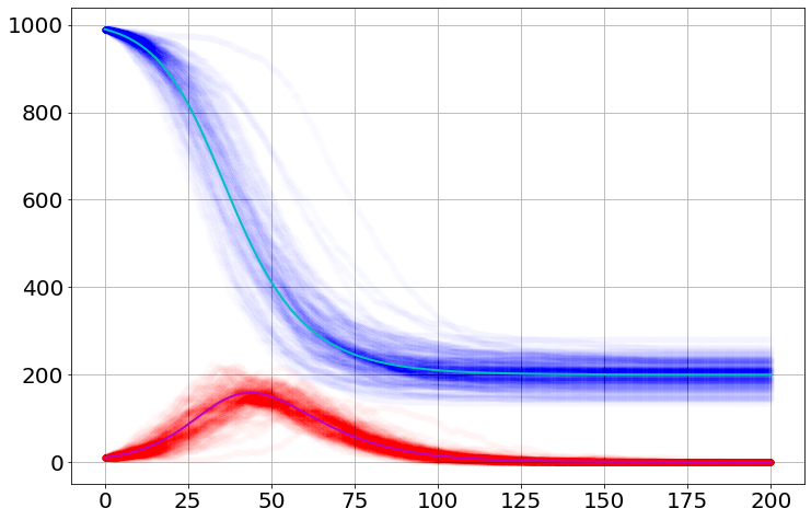
stoch_sim=sim=Stochastic_Simulation()
sim.add("-S+I",'β*S*I/N',S=So,I=Io)
sim.add("-I +R",'γ*I',R=0)
sim.add("N=S+I+R")
sim.params(β=β,γ=γ)
sim.run(200,Nsims=100)

for i in range(100):
    
    plot(sim.t,sim.S[i],'bo',alpha=0.05)
    plot(sim.t,sim.I[i],'ro',alpha=0.05)

plot(dynamic_sim.t,dynamic_sim.S,'c-')
plot(dynamic_sim.t,dynamic_sim.I,'m-')

print(sim.func_str)

100%|██████████| 100/100 [00:00<00:00, 981.58it/s]

@numba.jit(nopython=True)
def _propensity_function(population, args):
    S,I,R = population
    β,γ = args
    
    N=S+I+R
    
    return np.array([
        β*S*I/N,
        γ*I,
    ])

sim.extinction_times

array([173.34641097, 147.2142087 , 173.25806905, 139.46093989,
       141.46950986, 184.82415756, 177.24507978, 162.89244257,
       135.74875203, 142.12308477, 124.1452361 , 103.78449248,
       136.24764907, 141.64503261, 149.02049576, 154.08471155,
       144.36046575, 119.08888338, 126.56068263, 150.96714048,
       185.46651177, 137.75710629, 145.83280943, 161.45092743,
       135.52623017, 158.22300444, 116.4663216 , 142.45833271,
       131.58919096, 132.83514533, 158.67032537, 134.80159232,
       138.67325803, 145.34862087, 175.71694956, 168.1073566 ,
       138.83605961, 131.97878544, 132.29909228, 136.24188252,
       141.72408479, 149.24895424, 140.01290625, 134.00439041,
       128.82634577, 136.28831928, 121.92344439, 157.01860147,
       130.87983952, 190.04334344,  16.78030852, 175.76630482,
       116.42534703, 136.68052456,  -1.        , 136.61710555,
       183.78243168, 159.79643709, 148.65710129, 154.9672915 ,
       160.71863761, 166.15813836, 127.78792513, 139.85561763,
       177.64067511, 131.71662539, 126.83004396, 135.63721802,
       146.22285002, 170.34515699, 129.9729188 , 135.8394829 ,
       161.82999371, 154.39877207, 165.24073111,  -1.        ,
       134.46078024, 131.01546673, 121.36461215, 168.43992536,
       160.32262449, 144.3013475 , 199.74725228, 111.65022834,
       182.77090173, 113.66447594, 115.29110107, 138.87220524,
       175.75330356, 127.62963742, 137.38328691, 137.9071455 ,
       198.34523822, 144.94021945, 136.85662852, 166.1285249 ,
       176.12888724, 141.47111244, 146.1237378 , 177.42190037])

stoch_sim=sim=Stochastic_Simulation()
sim.add("+X",'X-X**2/N',X=10)
sim.add("-X",'X**2/N')
sim.params(N=10)
sim.run(50,num_iterations=101)

plot(sim.t,sim.X,'-o')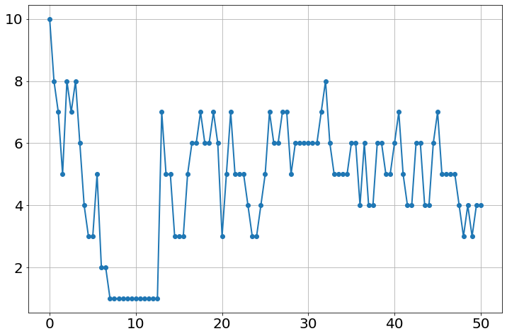

sim.extinction_times

array([-1])

Some Examples

Logistic

sim=Simulation()
sim.add("p'=a*p*(1-p/K)",100,plot=True)
sim.params(a=1.5,K=300)

sim.run(0,50)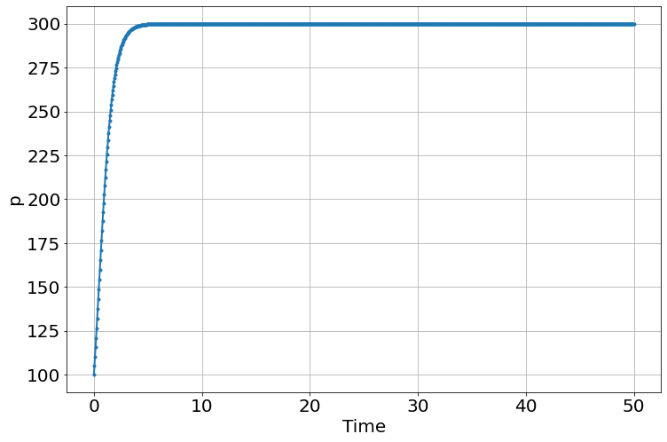

<Figure size 864x576 with 0 Axes>

sim=Simulation()
sim.add("x=a*x*(1-x)",0.11,plot=1)
sim.add("y=a*y*(1-y)",0.12,plot=1)
sim.params(a=3.5)

sim.run(0,50,discrete=True)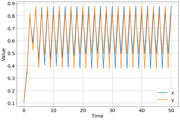

<Figure size 864x576 with 0 Axes>

Map

sim=Simulation('map')
sim.add("x=a*x*(1-x)",0.11)
figure(figsize=(12,8))
for a in linspace(.1,4,1200):
    sim.params(a=a)
    sim.run(0,1000)

    x=sim['x'][-100:]

    plot(a*ones(x.shape),x,'k.',markersize=.5)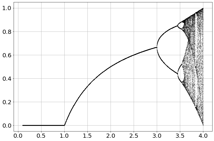

sim=Simulation('map')
sim.add("x=a*x*(1-x)",0.11)
figure(figsize=(12,8))
for a in linspace(3.2,4,1200):
    sim.params(a=a)
    sim.run(0,1000)

    x=sim['x'][-100:]

    plot(a*ones(x.shape),x,'k.',markersize=.5)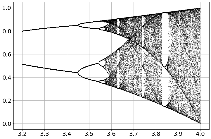

Repeat

sim=Simulation()
sim.add("growth_rate=a*(1-p/K)")
sim.add("p'=growth_rate*p",100)
sim.params(a=1.5,K=300)


result=sim.repeat(0,10,a=[1,2,3,4])
t=sim['t']

for res in result:
    p=res['p']
    plot(t,p)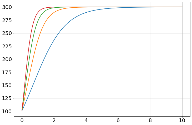

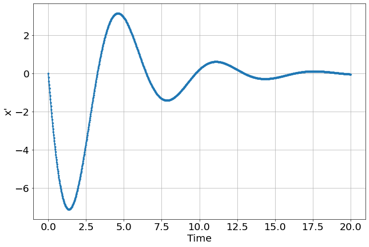
Higher Order

sim=Simulation()
sim.add("x''=-k*x/m -b*x'",[10,0],plot=True)
sim.params(k=1.0,m=1.0,b=0.5)

sim.run(0,20)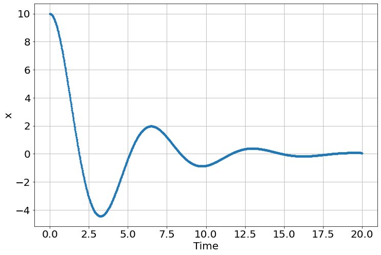

<Figure size 864x576 with 0 Axes>

phase_plot(sim,"x","x_p_")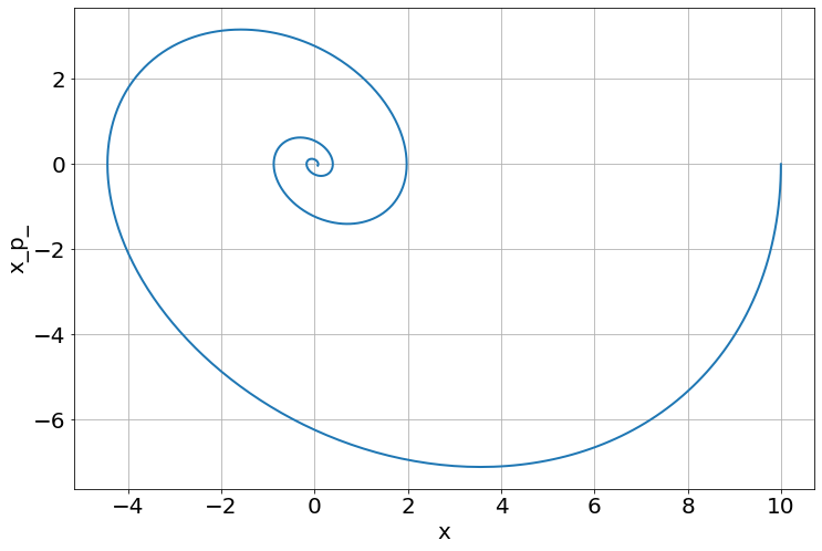

Exploring parameters

source

explore_parameters

 explore_parameters (sim, figsize=None, **kwargs)

sim=Simulation()
sim.add("p'=a*p*(1-p/K)",100,plot=True)
sim.add("K'=(50-K)/Kt",300,plot=False)
sim.params(a=1.5,Kt=30)

sim.run(0,50)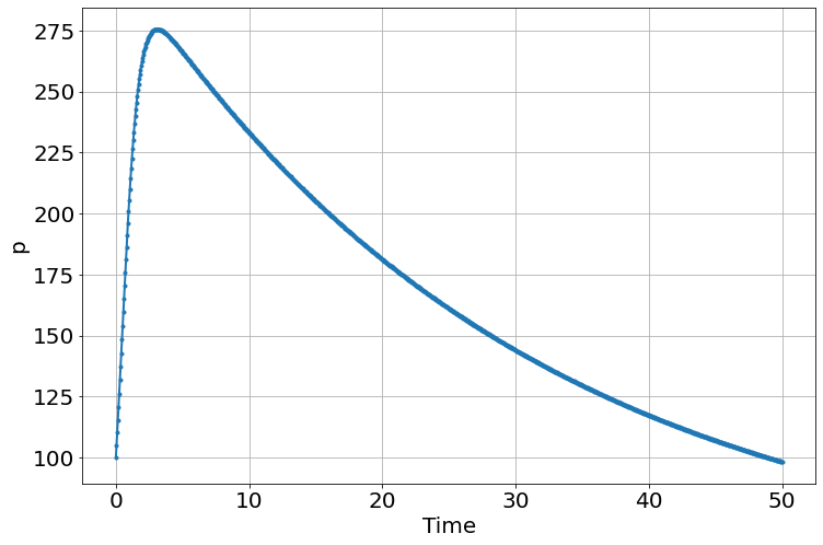

<Figure size 864x576 with 0 Axes>

explore_parameters(sim,Kt=linspace(10,100,10))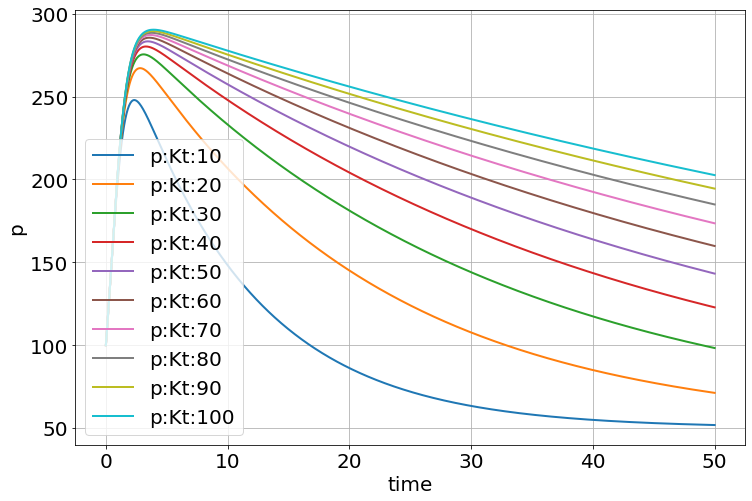

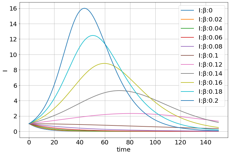
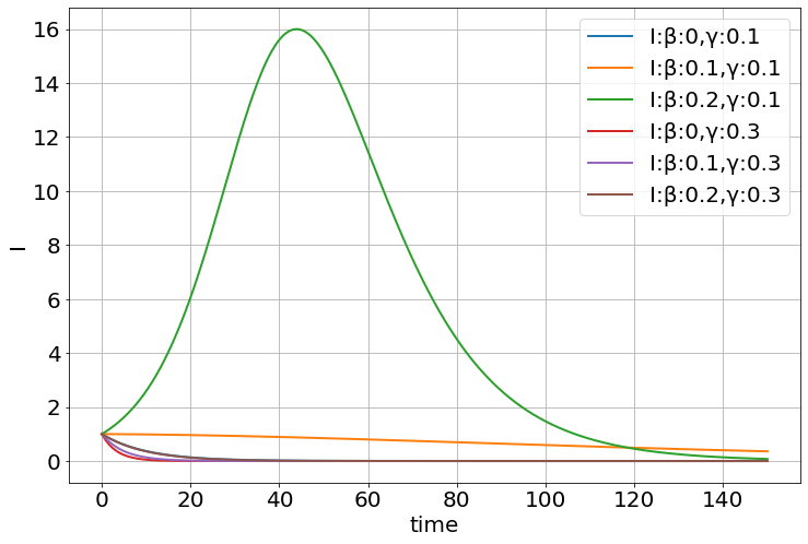
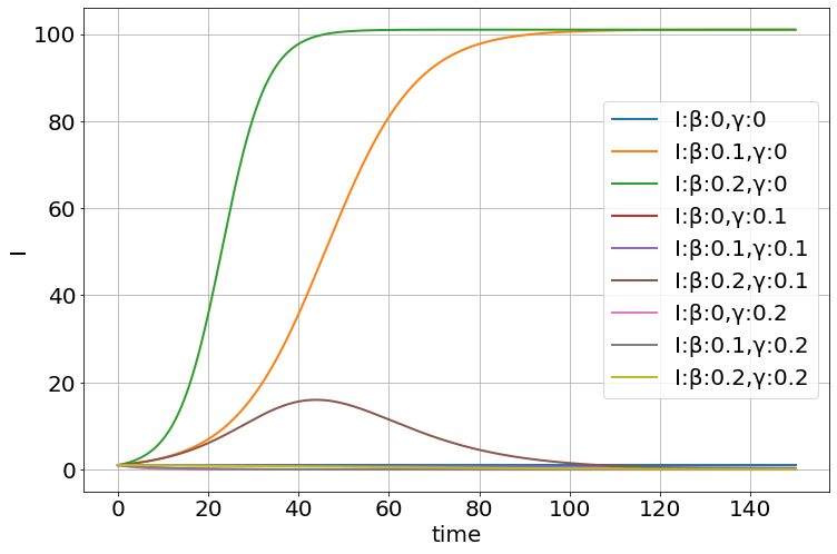
sim=Simulation()
sim.figsize=(8,4)
sim.add("S'=-β*S*I/N",100,plot=1)
sim.add("I'=+β*S*I/N - γ*I",1,plot=2)
sim.add("R'=+γ*I",0,plot=0)
sim.add("N=S+I+R",plot=0)
sim.params(β=0.2,γ=0.1)
sim.run(150)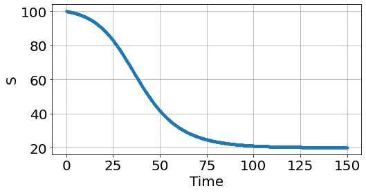

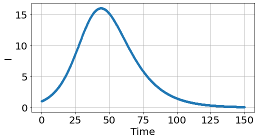
<Figure size 864x576 with 0 Axes>

explore_parameters(sim,figsize=(12,8),β=linspace(0,0.2,11))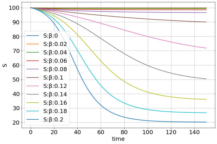

explore_parameters(sim,figsize=(12,8),β=[0,.1,.2,0,.1,.2],γ=[.1,.1,.1,.3,.3,.3])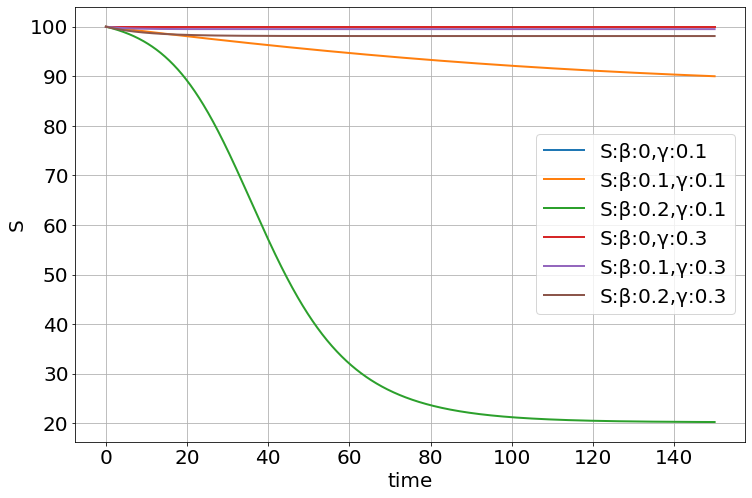

β,γ=meshgrid([0,.1,.2],[0,.1,.2])
explore_parameters(sim,figsize=(12,8),β=β,γ=γ)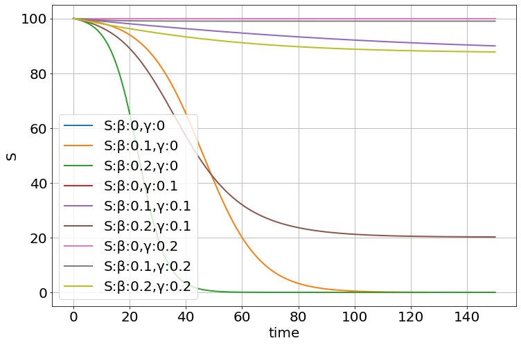

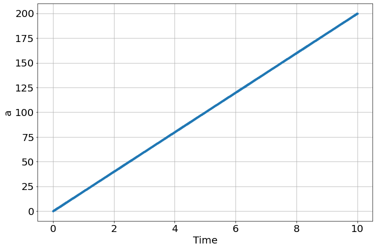
Functions of time

def a_vs_time(t):
    return 20*t
    
sim=Simulation()
sim.add("a=a_vs_time(t)",plot=1)
sim.add("y'=-a*y",100,plot=2)
sim.functions(a_vs_time)

sim.run(10)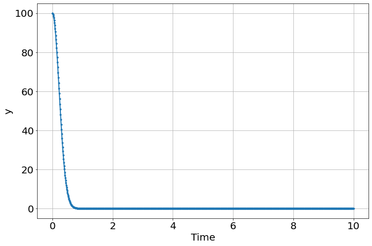

<Figure size 864x576 with 0 Axes>

Stochastic Simulation Examples

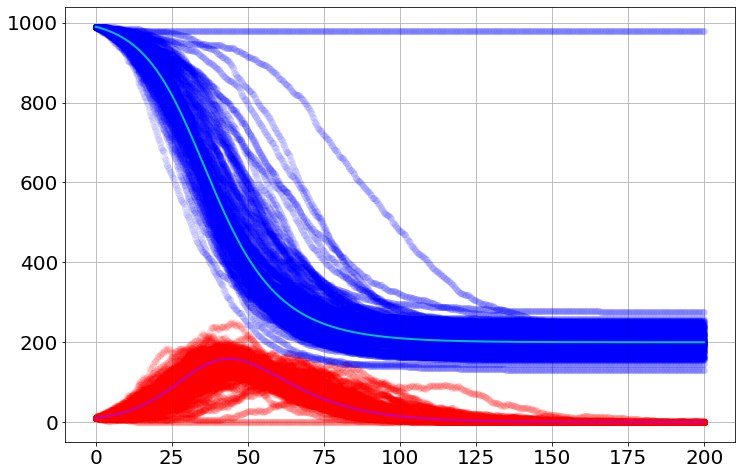
β=0.2
γ=0.1
So=990
Io=10

dynamic_sim=sim=Simulation()
sim.add("N=S+I+R")
sim.add("S'=-β*S*I/N",So)
sim.add("I'=+β*S*I/N-γ*I",Io)
sim.add("R'=+γ*I",0)
sim.params(β=β,γ=γ)
sim.run(200)


stoch_sim=sim=Stochastic_Simulation()
sim.add("-S+I",'β*S*I/N',S=So,I=Io)
sim.add("-I +R",'γ*I',R=0)
sim.add("N=S+I+R")
sim.params(β=β,γ=γ)
sim.run(200)

sim.run(200,Nsims=100)

for i in range(100):
    
    plot(sim.t,sim.S[i],'bo',alpha=0.005)
    plot(sim.t,sim.I[i],'ro',alpha=0.005)

plot(dynamic_sim.t,dynamic_sim.S,'c-')
plot(dynamic_sim.t,dynamic_sim.I,'m-')

100%|██████████| 100/100 [00:00<00:00, 1006.25it/s]

Preliminaries

patch

patch_to

copy_func

RedirectStdStreams

InterpFunction

array_wrap

from_values

Supporting functions for solving ODE and MAPS

simfunc

rk45

rkwrapper

rk4

rk2

euler

mapsolve

vector_field

phase_plot

Component

Examples of Components

The Simulation class is the primary one to use

Simulation

An alternate way of specifying the equations - stocks, inflows and outflows

Some useful functions

mse_from_sim

model

repeat

This is my solution to an age-old problem of storing data in loops

Storage

pso_fit_sim

swarm

particle

Stochastic Sims

Stochastic_Component

Stochastic_Simulation

Struct

Some Examples

Logistic

Map

Repeat

Higher Order

Exploring parameters

explore_parameters

Functions of time

Stochastic Simulation Examples

The `Simulation` class is the primary one to use