Expressing Ignorance

or why Bayes is not to be feared

Sat 09 May 2015 In #articles

I continue with my critique of the article Why I am not a Bayesian by Greg Mayer, where complains about the Bayesian approach to inference, and then espouses Maximum Likelihood methods. My previous post looked at the notion of prior vs likelihood, why we commonly use priors (even without always knowing it), and why they are necessary for hypothesis comparison. Here I wanted to focus on what I consider to be his biggest issue with the Bayes approach, and it is technical in nature. It happens to be the same issue that I've heard from others - how to specify priors. Mayer goes further, and says that the specification of ignorance is not well defined. I admit that there may be cases where that is true, but I haven't seen a convincing one yet. In the article he outlines the following argument against specifying initial ignorance with a prior:

Let’s look at simple genetic example: a gene with two alleles (forms) at the locus (say alleles $A$ and $a$). The two alleles have frequencies $p + q = 1$, and, if there are no evolutionary forces acting on the population and mating is at random, then the three genotypes ($AA$, $Aa$, and $aa$) will have the frequencies $p^2$, $2pq$, and $q^2$, respectively. If I am addressing the frequency of allele $a$, and I am a Bayesian, then I assign equal prior probability to all possible values of $q$, so

$P(q>.5) = 0.5$

But this implies that the frequency of the $aa$ genotype has a non-uniform prior probability distribution

$P(q^2>0.25) = 0.5$.

My ignorance concerning $q$ has become rather definite knowledge concerning $q^2$ (which, if there is genetic dominance at the locus, would be the frequency of recessive homozygotes; as in Mendel’s short pea plants, this is a very common way in which we observe the data). This apparent conversion of ‘ignorance’ to ‘knowledge’ will be generally so: prior probabilities are not invariant to parameter transformation (in this case, the transformation is the squaring of $q$). And even more generally, there will be no unique, objective distribution for ignorance. Lacking a genuine prior distribution (which we do have in the diagnosis example above), reasonable men may disagree on how to represent their ignorance. As Royall (1997) put it, “pure ignorance cannot be represented by a probability distribution”.

This example intrigued me because of its simplicity - it must have some solution. It also gave me an excuse to play with plotly, the online plotting program and emcee: The MCMC Hammer, both of which I had been meaning to get some practice in.

Summary

In summary,

Probability is a measure of our state of knowledge.
If we gain new information about our system, our state of knowledge changes, and thus the probabilities we assign must change.
Humans are bad an intuiting where information comes from in some cases, and thus often mistakenly think that two problems are equivalent when they are not.

Mayer's critique of priors with this genetic example is an example of point (3), and we outline that with a model analogy. In sum, the "apparent conversion of ‘ignorance’ to ‘knowledge’" that Greg Mayer is so concerned about is in fact not just apparent - it is explicit. This is not due to some arcane mathematics on priors, but to added information. What Mayer's considers to be equivalent situations - knowledge of only two possible states, and knowledge of the process that produces those states - are not equivalent at all.

The Model - Part 1

The model that I'm using comes in two steps. The first step concerns the observation of a system with two states, call them $+$ and $-$, and we want to infer from the observations of these states what the underlying probabilities, denoted $\theta_+$ and $\theta_-$ respectively, are. The observed data is something as simple as the number observed in one state vs the other, such as

\begin{eqnarray*} N_+ &=& 16 \\ N_- &=& 4 \\ N&\equiv& N_+ + N_- = 20 \end{eqnarray*}

The solution to this is achieved with a straightforward application of Bayes' rule:

\begin{eqnarray*} P(\theta_+|{\rm data}) &=& P({\rm data}|\theta_+)\times P(\theta_+)/K \\ P(\theta_-|{\rm data}) &=& \underbrace{P({\rm data}|-)}_{\rm likelihood}\times \underbrace{P(\theta_-)}_{\rm prior}/K \end{eqnarray*}

with normalization constant

\begin{eqnarray*} K\equiv P({\rm data}|\theta_+)\times P(\theta_+) + P({\rm data}|\theta_-)\times P(\theta_-) \end{eqnarray*}

and where the data is defined as

\begin{eqnarray*} {\rm data}&\equiv & \left\{ N_+,N \right\} \end{eqnarray*}

or equivalently

\begin{eqnarray*} {\rm data}&\equiv & \left\{ N_-,N \right\} \end{eqnarray*}

Although analytical solutions exist for this problem, I'll solve it with MCMC both to work on my implementation, but also to see how this could be applied to more challenging cases. To do this, we specify the log-prior and log-likelihoods for our parameters.

Prior

Notice that we know nothing about the origin of these states or the process which gives rise to these states, we only observe how many there are. Thus, we have total ignorance of the $\theta_-$ parameter, and we assign a uniform prior probability to reflect that.

$$ P(\theta_-) = \left\{\begin{array}{cl}1 & \mbox{ for } 0 \le \theta_- \le 1 \\ 0 & \mbox{ otherwise } \end{array}\right. $$

Likelihood

Since this is a straightforward Bernoulli process, we have for the likelihood

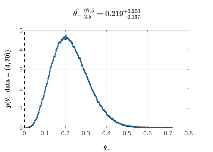
$$ P({\rm data}|\theta_-) = \left(\begin{array}{c}N \\ N_- \end{array}\right) \theta_{-}^{N_-}\times (1-\theta_-)^{N-N-} $$

Result

The resulting posterior for $\theta_-$ is

$\hat{\theta_-}|^{97.5}_{2.5}=0.219^{+0.200}_{-0.137}$

Again, clearly there is an analytic solution to this part, but that isn't the point. And I'm not sure whether the second part has an easy solution, but the MCMC approach is just as easy.

Model - Part 2

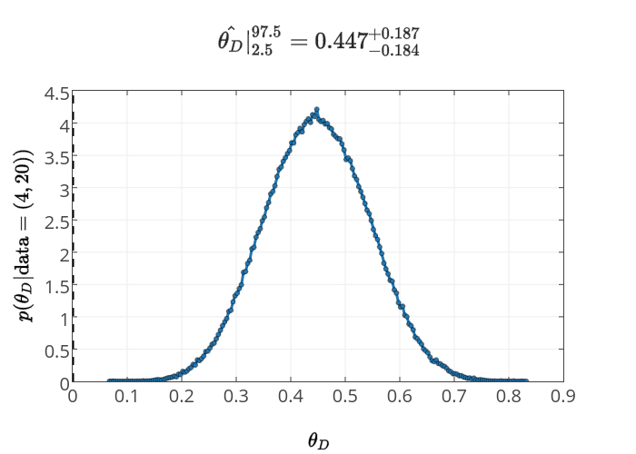
The second step in the model is when we get some detail of the process by which the $+$ and $-$ states are generated. Here is the recipe:

I flip a two identical thumbtacks, each of which can land with the point up ($U$) or down ($D$) - and I don't know anything about the probability of these two cases.
If either (or both) of the tacks lands with the point up, that is reported as the $+$ state. The only remaining case (i.e. both tacks land pointing down), is reported as the $-$ state.

We have, then, the following mapping:

$UU \rightarrow +$
$UD \rightarrow +$
$DU \rightarrow +$
$DD \rightarrow -$

The parallel with alleles should be obvious. By keeping it to a simple physical model, I avoid the extra complexities of genetic inheritance, and other biological processes.

This model, again, is a basic problem in probability, but note the following very important point:

Our knowledge of the system has changed, so our probabilities must also change.

The only difference is that our ignorance is now on $\theta_U$ and $\theta_D$, and the probabilities for the $+$ and $-$ states are derived from that,

\begin{eqnarray*} \theta_- &=& \theta_D^2 \\ \theta_+ &=& 1-\theta_- \end{eqnarray*}

Now we have posterior for the underlying parameters, such as $\theta_D$, as well as for the state parameters, such $\theta_-$, which are determined entirely from the underlying parameters. The posterior for $\theta_D$ is

$\hat{\theta_D}|^{97.5}_{2.5}=0.447^{+0.187}_{-0.184}$

while the posterior for $\theta_-$ in the Model 2 is

${\hat{\theta}_-}|^{97.5}_{2.5}=0.200^{+0.202}_{-0.131}$

Comparisons and conclusions

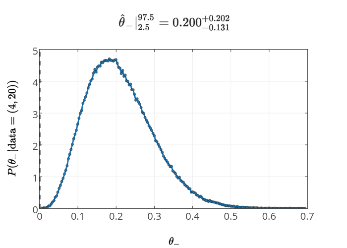
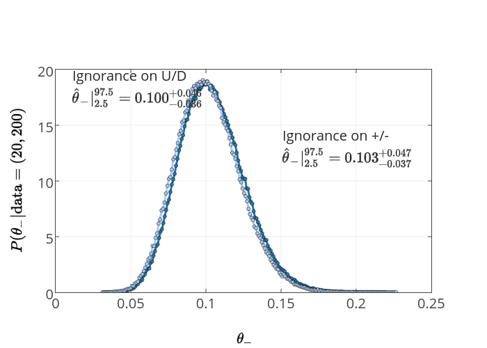
It's a bit more convenient to plot the consequences of Model 1 (ignorance in +/-) and Model 2 (ignorance in U/D), with the same data, both together on the same plot.

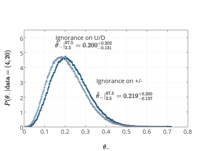
We can easily see that, although they are different, there is no practical difference between them given this data. For larger $N$ this difference gets less significant.

In sum, the "apparent conversion of ‘ignorance’ to ‘knowledge’" that Greg Mayer is so concerned about is in fact not just apparent - it is explicit. This is not due to some arcane mathematics on priors, but to added information. What Mayer's considers to be equivalent situations - knowledge of only two possible states, and knowledge of the process that produces those states - are not equivalent at all.

In practice, for this problem, it makes very little difference whether you think of things in terms of Model 1 or Model 2 except in the case of extremely rare underlying events. This is also as it should be - if you know that the process essentially hides the existence of itself (i.e. the recessive gene is not observed phenotypically) - then you would assign a lower probability for the phenotype than you would if you only knew that there were two possible states and knew nothing about the properties of recessive characteristics. To repeat, different states of knowledge require different probability assignments - this is a feature, not a bug.