
Gravitational Attraction
What would happen if two people out in space a few meters apart, abandoned by their spacecraft, decided to wait until gravity pulled them together? My initial thought was that …

A physics problem from a practice AP test came to my attention, when my daughter was in AP physics this past spring. I went over her solutions when she did the practice questions so that she would have another resource to explain the concepts involved. Due the new format this year, adjusting to the COVID-19 restrictions, there were only four such practice problems available to work from. Although the four questions were generally pretty good, I thought, the official solution to a quarter of one of the questions was simply incorrect.
It's a good example of how assumptions affect any problem, how a simple problem can get messy quickly, and how one can use computation to explore even a messy version of a physics problem. I was unable to solve the final part analytically because of an assumption the official solution made that was not explicitly stated in the problem. It turned out that this assumption was not physically reasonable, but was necessary in order to actually solve the problem.
The introduction to the problem is given here:
A student is given a spring that does NOT obey Hooke's Law. The student is told that the relationship between the magnitude of the force exerted by the spring and the magnitude of the spring's stretch or compression is given by the function \(F = Bx^3\) . The student wishes to determine whether this is the correct relationship between \(F\) and \(x\) and, if it is, to determine the value of \(B\).
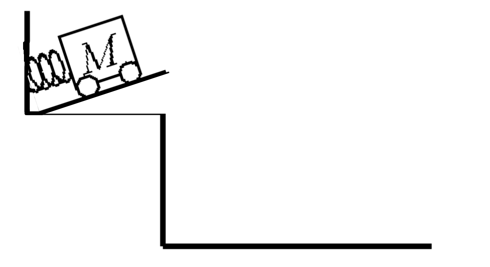
The student fixes the spring to a vertical wall just above a flat table, as shown above. The student also has a cart of known mass \(M\) that has light wheels and frictionless bearings. The student also has access to a meterstick and a scientific calculator that can perform four functions, exponents and roots, but cannot perform curve fitting or analyze lists of data.
(a) State the measurements that the student should make, and give each measurement a meaningful algebraic symbol.
(b) Describe the procedure that the student should follow in order to make the measurements necessary to accomplish the student's purpose.
(c) Explain how the student should use the measurements in order to accomplish the student's purpose. Explicitly explain how the relationship between \(F\) and \(x\) can be tested and the value of \(B\) determined.
(d) Suppose that the table is not level, so that the cart, upon becoming a projectile, has a sight upward launch angle. How would the true value of \(B\) compare to the value calculated by a student following your procedure and data analysis outlined above?
The official solution to the questions is posted is here: https://youtu.be/L1oIsHMB1RQ?t=1751
(a) State the measurements that the student should make, and give each measurement a meaningful algebraic symbol.
First I define the quantities, and derive expressions for the constants. I really answer this part
So, varying \(x_o\) and measuring the range, \(R\), we can determine \(B\).
(b) Describe the procedure that the student should follow in order to make the measurements necessary to accomplish the student's purpose.
Plotting \(R^2\) vs \(x_o^4\) the slope will be \(B\cdot h/4g\). Or better yet, plot \(\log(R)\) vs \(\log(x_o)\).
so the intercept will be \(\log\left(\frac{B\cdot h}{4g}\right)\).
(c) Explain how the student should use the measurements in order to accomplish the student's purpose. Explicitly explain how the relationship between \(F\) and \(x\) can be tested and the value of \(B\) determined.
The slope of the line from \(\log(R)\) vs \(\log(x_o)\) will determine the power of the spring energy function. Slope of \(4\) will confirm the \(x^3\) form of the force.
(d) Suppose that the table is not level, so that the cart, upon becoming a projectile, has a sight upward launch angle. How would the true value of \(B\) compare to the value calculated by a student following your procedure and data analysis outlined above?
This is where the official solution goes off the rails. He states that,
If launch angle is a little bit up, the value of the range [\(R\) in my notation, \(D\) in theirs] will be a little bit farther than they ideally would have been, so if you get a farther distance \(R\) than you should have gotten, then you would get a higher \(B\).
Hidden in this solution, but one not stated in the problem, is an assumption which we'll discuss later. We continue our solution of the ramp projectile. The range launched from a height \(h\) at an angle \(\theta\) is (https://en.wikipedia.org/wiki/Range_of_a_projectile),
this form doesn't look much like the flat-table range,
but you can show that they are the same in the limit \(\theta\rightarrow 0\),
which matches the form of \(R_o\).
It's not obvious that \(R_1\) is an increasing function of \(\theta\), as stated in the solution (e.g. angle goes up, the range goes up) but numerically it is easy to demonstrate,
B=2  # true value
x0=1.1
m=0.01
h=20
g=10

θ=linspace(0.001,60,100)

U=B*x0**4/4
KE=U
v=sqrt(KE*2/m)

R0=sqrt(v**2*2*h/g)*ones(len(θ))
R1=v**2/2/g*(1+sqrt(1+2*g*h/v**2/sin(radians(θ))**2))*sin(radians(2*θ))

θ_at_max=arcsin(sqrt(2)*v*sqrt(1/(g*h + v**2))/2)
θ_at_max2=arcsin(1/sqrt(2)*1/sqrt(1+2*g*h*m/B/x0**4))

B_est0=R0**2*g*m/(x0**4*h)
B_est1=R1**2*g*m/(x0**4*h)
figure(figsize=(16,6))
subplot(1,2,1)
plot(θ,R0,label='No Ramp')
plot(θ,R1,label='With Ramp')

vlines(degrees(θ_at_max),*ylim(),ls=':')
vlines(degrees(θ_at_max2),*ylim(),ls='--',lw=1,color='r')

ylabel('Range')
xlabel('Angle')
legend()


subplot(1,2,2)
plot(θ,B_est0,label='No Ramp')
plot(θ,B_est1,label='With Ramp')
vlines(degrees(θ_at_max),*ylim(),ls=':')
ylabel('$B$')
xlabel('Angle')
legend()
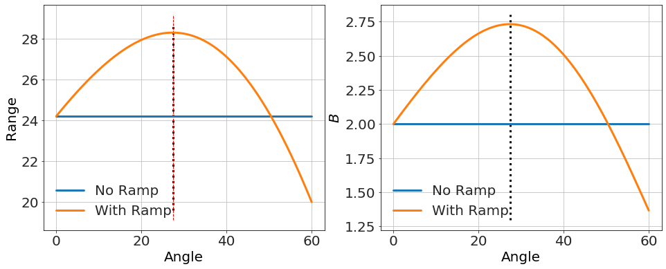
As you can see, for small angle, the range increases with angle before decreasing again for steep angles. So far, so good. You wouldn't expect a student on a test to do the next parts, but I wasn't convinced that the assumption made in the solution held in all cases, or that there wasn't some range of parameters for which the simplistic "angle goes up, range goes up" would hold experimentally. So, I continued the analysis in as much deatil as I could.
What is shown in the plot is that above some critical angle, the range starts going down. We expect that, because obviously if you had a ramp of \(\theta=90^\circ\) you'd have no range. But what if that critical angle was somehow small, like \(2^\circ\)? One might miss it experimentally if you were measuring, say, every \(5^\circ\). But could this ever happen in this simple system? Let's see.
The critical angle that gives the maximum range is determined analytically from,
import sympy as sym
v,g,h,θ,x_o,B,m=sym.symbols("v g h θ x_o B m")
R1=v**2/2/g*(1+sym.sqrt(1+2*g*h/v**2/sym.sin(θ)**2))*sym.sin(2*θ)
display(R1)
\(\displaystyle \frac{v^{2} \left(\sqrt{\frac{2 g h}{v^{2} \sin^{2}{\left(θ \right)}} + 1} + 1\right) \sin{\left(2 θ \right)}}{2 g}\)
df=sym.diff(R1,θ)
soln=sym.solve(sym.simplify(df),θ)
soln
[-asin(sqrt(2)*v*sqrt(1/(g*h + v**2))/2),
 asin(sqrt(2)*v*sqrt(1/(g*h + v**2))/2)]
sin_θ_at_max=sym.sqrt(2)*v*sym.sqrt(1/(g*h + v**2))/2
display(sin_θ_at_max)
\(\displaystyle \frac{\sqrt{2} v \sqrt{\frac{1}{g h + v^{2}}}}{2}\)
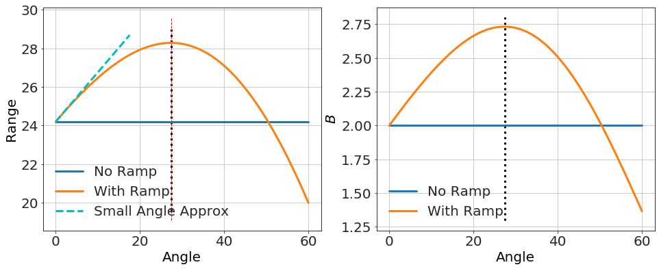
The slope near \(\theta=0\) is positive, as can be derived by
Applying small angle approximation for the trigonometric functions (e.g. \(\sin\theta\sim \theta\), \(\cos\theta \sim 1\)) we get
which is positive. Checking that this works numerically as well,
B=2  # true value
x0=1.1
m=0.01
h=20
g=10

θ=linspace(0.001,60,100)

U=B*x0**4/4
KE=U
v=sqrt(KE*2/m)

R0=sqrt(v**2*2*h/g)*ones(len(θ))
R1=v**2/2/g*(1+sqrt(1+2*g*h/v**2/sin(radians(θ))**2))*sin(radians(2*θ))

θ_at_max=arcsin(sqrt(2)*v*sqrt(1/(g*h + v**2))/2)
θ_at_max2=arcsin(1/sqrt(2)*1/sqrt(1+2*g*h*m/B/x0**4))

B_est0=R0**2*g*m/(x0**4*h)
B_est1=R1**2*g*m/(x0**4*h)
figure(figsize=(16,6))
subplot(1,2,1)
plot(θ,R0,label='No Ramp')
plot(θ,R1,label='With Ramp')

x=radians(θ[:30])
m=v**2/g
b=R0[0]
y=m*x+b
plot(θ[:30],y,'c--',label='Small Angle Approx')


vlines(degrees(θ_at_max),*ylim(),ls=':')
vlines(degrees(θ_at_max2),*ylim(),ls='--',lw=1,color='r')

ylabel('Range')
xlabel('Angle')
legend()


subplot(1,2,2)
plot(θ,B_est0,label='No Ramp')
plot(θ,B_est1,label='With Ramp')
vlines(degrees(θ_at_max),*ylim(),ls=':')
ylabel('$B$')
xlabel('Angle')
legend()
Given the symmetry, the point where the range starts decreasing with angle is at twice this angle. Subsituting in the launch speed for the flat table, \(v_o^2 = \frac{B x_o^4}{2 m}\), we get something interesting.
sin_θ_at_max.subs(v,sym.sqrt(B*x_o**4/2/m)).simplify()
\(\displaystyle \frac{\sqrt{2} v \sqrt{\frac{1}{g h + v^{2}}}}{2}\)
yielding,
the point here is that, while technically true that the range is an increasing function of \(\theta\) for small \(\theta\), the turning point can be made arbitrarily small in certain parameter regions (e.g. small \(B\), small \(x_o\), large \(m\), etc...). For instance,
B=2  # true value
x0=0.1
m=0.01
h=20
g=10

θ=linspace(0.001,3,100)

U=B*x0**4/4
KE=U
v=sqrt(KE*2/m)

R0=sqrt(v**2*2*h/g)*ones(len(θ))
R1=v**2/2/g*(1+sqrt(1+2*g*h/v**2/sin(radians(θ))**2))*sin(radians(2*θ))

θ_at_max=arcsin(sqrt(2)*v*sqrt(1/(g*h + v**2))/2)
θ_at_max2=arcsin(1/sqrt(2)*1/sqrt(1+2*g*h*m/B/x0**4))

B_est0=R0**2*g*m/(x0**4*h)
B_est1=R1**2*g*m/(x0**4*h)
figure(figsize=(16,6))
subplot(1,2,1)
plot(θ,R0,label='No Ramp')
plot(θ,R1,label='With Ramp')

x=radians(θ[:30])
m=v**2/g
b=R0[0]
y=m*x+b
plot(θ[:30],y,'c--',label='Small Angle Approx')


vlines(degrees(θ_at_max),*ylim(),ls=':')
vlines(degrees(θ_at_max2),*ylim(),ls='--',lw=1,color='r')

ylabel('Range')
xlabel('Angle')
legend()


subplot(1,2,2)
plot(θ,B_est0,label='No Ramp')
plot(θ,B_est1,label='With Ramp')
vlines(degrees(θ_at_max),*ylim(),ls=':')
ylabel('$B$')
xlabel('Angle')
legend()
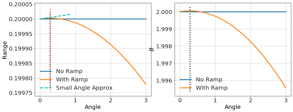
So the claim that "range increases with angle" could be missed experimentally if the turning point is smaller than the ramp angle. To the person making the measurement, the range would decrease with angle. Still, technically, that claim is true...assuming the same launch speed.
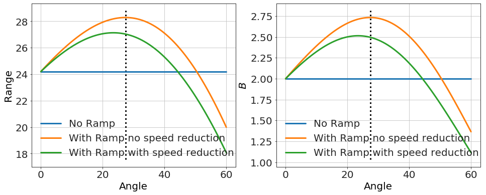
This brings us to the real problem with the given solution: the launch speed for the ramp case is not the same as the flat case. The spring gives the same amount to the kinetic energy, but it does so by having the block move up the ramp as the spring expands. Thus, the total kinetic energy of the block upon launch depends on the angle,
This leads to a range equation like the one above for \(R_1\), but with an angle-dependent speed. We'll call this range \(R_2\).
(https://en.wikipedia.org/wiki/Range_of_a_projectile),
which is a whole lot messier, and the slope is difficult to attain analytically. Numerically however, it is easy to see the effect. Depending on the parameters, the range could increase or decrease with angle.
Here's an example with increasing with angle.
B=2  # true value
x0=1.1
m=0.01
h=20
g=10

θ=linspace(0.001,60,100)

U=B*x0**4/4
KE=U
v=sqrt(KE*2/m)
v_o=v

R0=sqrt(v**2*2*h/g)*ones(len(θ))
R1=v**2/2/g*(1+sqrt(1+2*g*h/v**2/sin(radians(θ))**2))*sin(radians(2*θ))

θ_at_max=arcsin(sqrt(2)*v*sqrt(1/(g*h + v**2))/2)

KE=U-m*g*x0*sin(radians(θ))
v=sqrt(KE*2/m)
R2=v**2/2/g*(1+sqrt(1+2*g*h/v**2/sin(radians(θ))**2))*sin(radians(2*θ))


B_est0=R0**2*g*m/(x0**4*h)
B_est1=R1**2*g*m/(x0**4*h)
B_est2=R2**2*g*m/(x0**4*h)
figure(figsize=(16,6))
subplot(1,2,1)
plot(θ,R0,label='No Ramp')
plot(θ,R1,label='With Ramp no speed reduction')
plot(θ,R2,label='With Ramp with speed reduction')


vlines(degrees(θ_at_max),*ylim(),ls=':')
ylabel('Range')
xlabel('Angle')
legend()


subplot(1,2,2)
plot(θ,B_est0,label='No Ramp')
plot(θ,B_est1,label='With Ramp no speed reduction')
plot(θ,B_est2,label='With Ramp with speed reduction')
vlines(degrees(θ_at_max),*ylim(),ls=':')
ylabel('$B$')
xlabel('Angle')
legend()
Here's an example with decreasing with angle.
B=2  # true value
x0=.4
m=0.01
h=20
g=10

θ=linspace(0.001,10,100)

U=B*x0**4/4
KE=U
v=sqrt(KE*2/m)

R0=sqrt(v**2*2*h/g)*ones(len(θ))
R1=v**2/2/g*(1+sqrt(1+2*g*h/v**2/sin(radians(θ))**2))*sin(radians(2*θ))


KE=U-m*g*x0*sin(radians(θ))
v=sqrt(KE*2/m)
R2=v**2/2/g*(1+sqrt(1+2*g*h/v**2/sin(radians(θ))**2))*sin(radians(2*θ))

B_est0=R0**2*g*m/(x0**4*h)
B_est1=R1**2*g*m/(x0**4*h)
B_est2=R2**2*g*m/(x0**4*h)
figure(figsize=(16,6))
subplot(1,2,1)
plot(θ,R0,label='No Ramp')
plot(θ,R1,label='With Ramp no speed reduction')
plot(θ,R2,label='With Ramp with speed reduction')


ylabel('Range')
xlabel('Angle')
legend()


subplot(1,2,2)
plot(θ,B_est0,label='No Ramp')
plot(θ,B_est1,label='With Ramp no speed reduction')
plot(θ,B_est2,label='With Ramp with speed reduction')
ylabel('$B$')
xlabel('Angle')
legend()
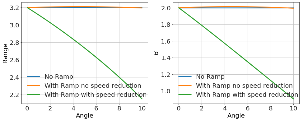
This problem was a very nice problem for the AP test until the last section. A hidden assumption -- that the launch speed is unaffected by the ramp -- would have made it much better and avoided any possible complications. However it's not a great assumption given the way the table and block are set up -- there is definitely a gravitational component to energy picked up along the ramp. Without this simplifying assumption the effect is much more complicated.
Gravitational Attraction
What would happen if two people out in space a few meters apart, abandoned by their spacecraft, decided to wait until gravity pulled them together? My initial thought was that …
A Simple Physics Problem Gets Messy
A physics problem from a practice AP test came to my attention, when my daughter was in AP physics this past spring. I went over her solutions when she did …

Skepticism and Dubious Medical Procedures
In my discussion with Jonathan McLatchie on the Still Unbelievable podcast, I said that there hasn’t been a verified miracle claim even since Hume’s essay on miracles. Here I look into the papers he references in response.
What problems are you interested in? How can I help?