Simulating Stochastic Processes

Gillespie Algorithm

Fri 07 January 2022 In #science

In this post we are going to explore the simulation of stochastic (i.e. random) processes, and work our way to understanding how the Gillespie algorithm works. We'll be using mostly straightforward Python, except for my Storage class from https://bblais.github.io/posts/2020/Feb/24/common-python-pattern-building-up-lists-to-plot/ and some default plotting preferences specified in https://raw.githubusercontent.com/bblais/Python-for-Science/master/science/science.mplstyle.

Imports

%pylab inline
style.use('science.mplstyle')
from Memory import Storage

A simple problem

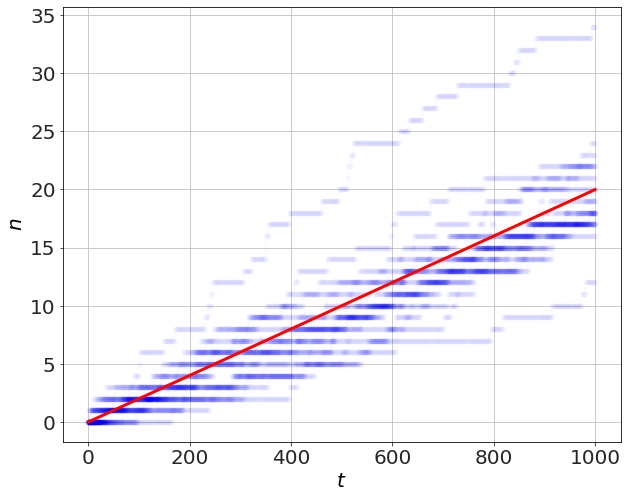
In this first problem, we have a process that occurs with probability $p=0.02$ per second. When an event happens, the number $n$ is incremented by 1. The average linear rate of increase will be the same as $p$ .

number_of_simulations=20
dt=1.0
p=0.02
for _ in range(number_of_simulations):
    S=Storage()
    t=0
    n=0
    S+=t,n
    while t<1000:
        if rand()<p*dt:
            n+=1

        t+=dt

        S+=t,n

    t,n=S.arrays()
    plot(t,n,'b-o',alpha=0.01)


plot(t,p*t,'r-')


ylabel('$n$')
xlabel('$t$')

To motivate the faster algorithm, let's run a bunch of simulations, and record the time to the first event only. Then count up how many events happen at the various times.

S=Storage()

N=50000
p=0.03
for _ in range(N):

    t=0
    while True:
        if rand()<p:
            break

        t+=1

    S+=t,

t=S.arrays()

n,tn,h=hist(t,200);
xlabel('time to first event')
ylabel('number of events')


slope,intercept=polyfit(tn[:100],log(n[:100]),1)
plot(tn[:100],exp(slope*tn[:100]+intercept),'r-')

λ=p
plot(tn,exp(-λ*tn)*n[0],'k--',lw=5)

Pasted image 20220106220712.png

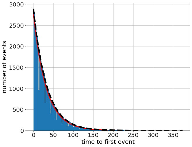
which looks exponential, so we compare it to an exponentiial fit (linear fit to the log) and an exponential with a decay factor $\lambda=p$ . The fit is quite good!

To normalize analytically (and make it a proper probability function), we need to make sure that the integral over $t$ is 1,

$\begin{aligned} p(t)&= p_o e^{-\lambda t}\\ \int_0^{+\infty} p_o e^{-\lambda t} dt &=1 \\ \left.\left(\frac{1}{-\lambda}\right)p_o e^{-\lambda t}\right|^{+\infty}_{0} &=1 \\ 0 - \left(\frac{1}{-\lambda}\right)p_o &=1 \\ p_o &=\lambda \end{aligned}$ therefore the distribution is

$p(t) = \lambda e^{-\lambda t}$ which can be seen here https://en.wikipedia.org/wiki/Exponential_distribution

Towards Gillespie

Instead of flipping the coin every millisecond (i.e. constant time), we can randomly pick a time from an exponential distribution -- the time to the next event (i.e. dynamic time).

def constant_time(N=20,n0=0,t_max=1000,p=0.02,dt=1):
    S_mat=[]
    for _ in range(N):
        S=Storage()
        t=0
        n=n0
        S+=t,n
        while t<t_max:
            if rand()<p*dt:
                n+=1

            t+=dt

            S+=t,n

        S_mat.append(S)

    return S_mat

and

def dynamic_time(N=20,n0=0,t_max=1000,p=0.02,dt=1):
    S_mat=[]
    for _ in range(N):
        S=Storage()
        t=0
        n=n0
        S+=t,n
        while t<t_max:
            λ=p
            t_next=np.random.exponential(1/λ)

            t=t+t_next
            S+=t,n

            n+=1
            S+=t,n


        S_mat.append(S)

    return S_mat

to get

figure(figsize=(12,10))
subplot(2,1,1)

for S in constant_time():
    t,n=S.arrays()
    plot(t,n,'b-o',alpha=0.01)

ylabel('$n$')
title('Constant Time')
xlim([0,1000])
gca().set_xticklabels([]);


subplot(2,1,2)

for S in dynamic_time():
    t,n=S.arrays()
    plot(t,n,'b-o',alpha=0.1)

ylabel('$n$')
xlabel('$t$')
title('Dynamic Time')
xlim([0,1000])

Pasted image 20220106221326.png

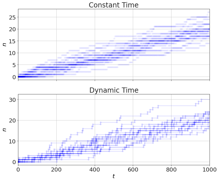
Timing this, we get more than 10x faster with the dynamic time. This would be more if the rates were lower.

%timeit S_mat=constant_time();

18.8 ms ± 614 µs per loop (mean ± std. dev. of 7 runs, 10 loops each)

%timeit S_mat=dynamic_time();

1.39 ms ± 29.3 µs per loop (mean ± std. dev. of 7 runs, 1000 loops each)

Gillespie

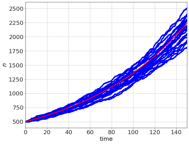
We now can extend the problem to the next simplest case, where two types of events can happen, say a birth probability and a death probability. This extension will have two added complexities from the previous example: 1. more than one type of event 2. the probabilities for those events, which determine the rates, depend on the variables and thus depend on time

In the simple birth-death process we have,

$\begin{aligned} p_\text{birth}&=b\cdot n\\ p_\text{death}&=d\cdot n\\ \end{aligned}$ where $b$ and $d$ are the per-capita probability for a birth or death, respectively, and where a birth results in $n\rightarrow n+1$ and a death results in $n\rightarrow n-1$ . The Gillespie algorithm proceeds in two steps 1. generate the next time (like above) for some event using the sum of the rates of all of the possible events 2. randomly choose one of the possible events, weighted by their prospective rates -- faster processes chosen more often

In code this could look like

no=5
b=0.03
d=0.02
for _ in range(20):
    S=Storage()

    n=no
    t=0
    S+=t,n
    t_max=200
    while t<t_max:
        pb=b*n
        pd=d*n

        rates=[pb,pd]
        total_rates=sum(rates)

        if not total_rates:
            break
        time_next = np.random.exponential(1 / total_rates)
        r=np.random.rand()*total_rates

        t+=time_next
        S+=t,n
        if r<pb:
            n+=1
        else:
            n-=1

        S+=t,n

    S+=t,n
    t,n=S.arrays()
    plot(t,n,'b.-',alpha=0.1)


t=linspace(0,t_max,100)
plot(t,no*exp((b-d)*t),'r-')    
xlabel('time')
ylabel('$n$')
xlim([0,t_max])

Pasted image 20220107080030.png

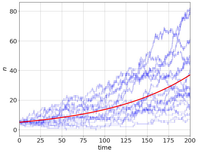
for large N, this should look like the solution

$\frac{dn}{dt}=b\cdot n - d\cdot n$ which will be exponential (population growth), $n=n_o e^{(b-d)\cdot t}$ which you can see in the red. In the small- $N$ case (like the one above, starting with $n=5$ , there is a lot of variation, but the average is the exponential curve. Changing $n_o=500$ we can see the variation reduces considerably.

Pasted image 20220107080819.png

Gillespie with SIR Model

As a final example we look at a probabilistic SIR model. In this model we have three sub-populations or compartments, $S$ , $I$ , and $R$ for Susceptible, Infected, and Recovered. The Susceptible become infected at a rate of $\beta S I$ and the Infected recover at a rate of $\gamma I$ . Another way to write this is as two possible events.

$\begin{aligned} S,I &\stackrel{\beta S I}{\longrightarrow} S-1, I+1\\ I,R &\stackrel{\gamma I}{\longrightarrow} I-1, R+1\\ \end{aligned}$ So, Gillespie follows by

generate the next time (like above) for some event (e.g. one of the two above) using the sum of the rates of all of the possible events
randomly choose one of the possible events, weighted by their prospective rates -- faster processes chosen more often

number_of_sims=100

for _ in range(number_of_sims):

    Io=1
    N=100
    tmax=100


    Io=1
    β=1
    γ=0.5


    t=0.0
    ni=Io
    ns=N-ni
    nr=0

    S=Storage()
    S+=t,ns,ni,nr    

    tw=0.0
    while (t < tmax):
        w1=β*ns*ni/N  # infect
        w2=γ*ni # recover
        w=w1+w2    

        tn=-log(rand())/w  # when's the next thing happening?
        t=t+tn
        r=rand()*w  # which thing happened?
        if (r < w1):
            ns-=1
            ni+=1
        else: 
            nr+=1
            ni-=1


        S+=t,ns,ni,nr

        if ni==0:
            break


    t,ns,ni,nr=S.arrays()

    plot(t,ns,'b',alpha=0.1)
    plot(t,ni,'g',alpha=0.1)
    plot(t,nr,'r',alpha=0.1)    



# these numbers taken from a pyndamics simulation, just for comparison
t,S,I,R=(array([ 0.        ,  1.57894737,  3.15789474,  4.73684211,  6.31578947,
         7.89473684,  9.47368421, 11.05263158, 12.63157895, 14.21052632,
        15.78947368, 17.36842105, 18.94736842, 20.52631579, 22.10526316,
        23.68421053, 25.26315789, 26.84210526, 28.42105263, 30.        ]),
         array([99.        , 96.68233609, 92.04102645, 83.73584541, 71.42053096,
                57.24621795, 44.66960674, 35.51429297, 29.55644131, 25.85923582,
                23.59619256, 22.21121513, 21.36043856, 20.83578683, 20.51122022,
                20.31000289, 20.18506816, 20.10742367, 20.05914037, 20.02910249]),
         array([ 1.        ,  2.13320482,  4.31469633,  7.89149267, 12.25267231,
                15.36581863, 15.53893182, 13.22645672, 10.00259897,  7.01814482,
                 4.70207514,  3.0626549 ,  1.96059584,  1.2418213 ,  0.78139042,
                 0.48968045,  0.30609591,  0.19103806,  0.11911362,  0.07422209]),
         array([ 0.        ,  1.18445909,  3.64427722,  8.37266192, 16.32679674,
                27.38796342, 39.79146144, 51.25925031, 60.44095972, 67.12261936,
                71.7017323 , 74.72612997, 76.6789656 , 77.92239186, 78.70738935,
                79.20031666, 79.50883592, 79.70153827, 79.821746  , 79.89667542]))


# these are here to get the legend with the right colors
plot(t,S,'b-',label='S')
plot(t,I,'g-',label='I')
plot(t,R,'r-',label='R')    
legend()

xlabel('time')
ylabel('number')

Pasted image 20220107082918.png

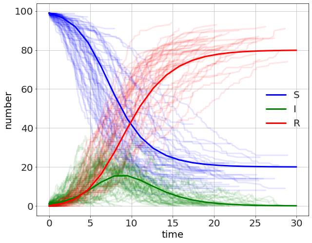
The comparison is made with a continuous version of the model using the pyndamics3 library. We will see later that we can use pyndamics3 to do stochastic algorithms as well.