
Gravitational Attraction
What would happen if two people out in space a few meters apart, abandoned by their spacecraft, decided to wait until gravity pulled them together? My initial thought was that …
In #math

This is another in the series of "Statistics 101" examples solved with MCMC. The previous in the series can be found here. In all of these posts I'm going to use a python library I make for my science-programming class, stored on github, and the emcee library. Install like:
pip install "git+git://github.com/bblais/sci378" --upgrade
pip install emcee
In this example, like the last one, there is some true value, we call \(\mu\). The \(N\) data points we have, \(\{x_i\}\), consist of that true value with added independent, normally-distributed noise of unknown scale, \(\sigma\).
For a Bayesian solution, we need to specify the likelihood function -- how our model produces the data -- and the prior probability for the parameters. The likelihood function is determined exactly as before,
but with unknown scale, \(\sigma\).
In the "Statistics 101" examples, the results are typically equivalent to uniform priors on the location parameters, but Jeffreys priors on scale parameters, so we'll assume uniform priors on \(\mu\) and Jeffreys priors on \(\sigma\)
In this example, like the last one, there is some true value, we call \(\mu\), with normally-distributed noise but this time with unknown scale, \(\sigma\). The likelihood function is determined identically as before,
known \(\sigma\)
and we'll assume uniform priors on \(\mu\). The prior for \(\sigma\), which we must now estimate, is taken to be a Jeffreys prior. This prior is uniform in \(\log \sigma\) or, in other words, uniform in scale.
def lnlike(data,μ):
    # known σ
    x=data
    return lognormalpdf(x,μ,σ)

data=array([12.0,14,16])
model=MCMCModel(data,lnlike,
                μ=Uniform(-50,50),
                σ=Jeffreys(),
)
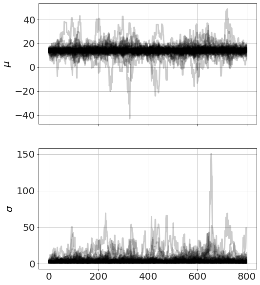
Now we run MCMC, plot the chains (so we can see it has converged) and look at distributions,
model.run_mcmc(800,repeat=3)
model.plot_chains()
Sampling Prior...
Done.
0.27 s
Running MCMC 1/3...
Done.
2.63 s
Running MCMC 2/3...
Done.
2.79 s
Running MCMC 3/3...
Done.
2.47 s
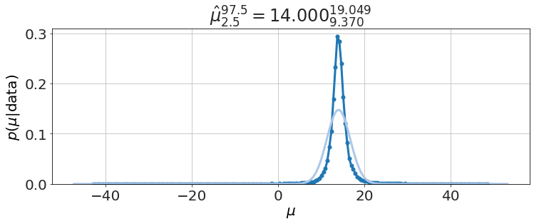
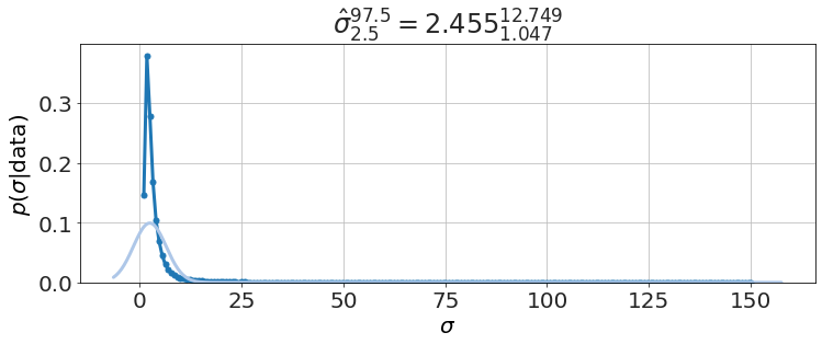
model.plot_distributions()
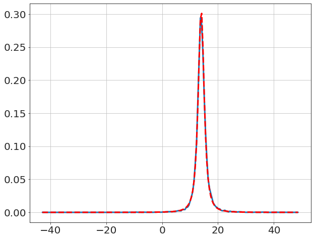
We compare to textbook solution for \(\mu\) (i.e. Student t-distribution),
x,y=model.get_distribution('μ')

plot(x,y,'-')
μ̂=mean(data)
N=len(data)

σμ=std(data,ddof=1)/sqrt(N)
y_pred=[exp(logtpdf(_,N-1,μ̂,σμ)) for _ in x]
plot(x,y_pred,'r--')
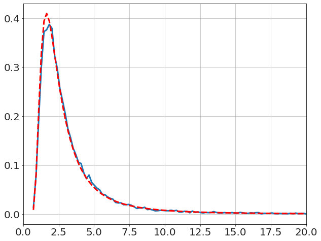
and the textbook solution for \(\sigma\) (i.e. Chi-square),
x,y=model.get_distribution('σ',bins=800)
plot(x,y,'-')

V=((data-data.mean())**2).sum()
logp=-N*log(x)-V/2/x**2
y_pred=exp(logp)
dx=x[1]-x[0]
y_pred=y_pred/y_pred.sum()/dx

plot(x,y_pred,'r--')
xlim([0,20])
We can easily find the tail-area probability, the Bayesian equivalent to Student-t test, for \(\mu\),
model.P("μ>15")
0.037066666666666664
and for \(\sigma\), the Bayesian equivalent to Chi-squared test,
model.P("σ<1")
0.01985
Gravitational Attraction
What would happen if two people out in space a few meters apart, abandoned by their spacecraft, decided to wait until gravity pulled them together? My initial thought was that …

A Simple Physics Problem Gets Messy
A physics problem from a practice AP test came to my attention, when my daughter was in AP physics this past spring. I went over her solutions when she did …

Skepticism and Dubious Medical Procedures
In my discussion with Jonathan McLatchie on the Still Unbelievable podcast, I said that there hasn’t been a verified miracle claim even since Hume’s essay on miracles. Here I look into the papers he references in response.
What problems are you interested in? How can I help?