
Gravitational Attraction
What would happen if two people out in space a few meters apart, abandoned by their spacecraft, decided to wait until gravity pulled them together? My initial thought was that …
In #math
This is another in the series of "Statistics 101" examples solved with MCMC. Others in the series:
In all of these posts I'm going to use a python library I make for my science-programming class, stored on github, and the emcee library. Install like:
pip install "git+git://github.com/bblais/sci378" --upgrade
pip install emcee
In this example the data take the form of a number of "successes", \(h\), in a total number of "trials", \(N\), and we want to estimate the proportion, \(\theta\). This could be the number of heads observed in \(N\) coin flips and we want to estimate the bias in the coin -- what is the probability that it flips heads. In fact, the data I will use below is from Lindley, 1976. "Inference for a Bernoulli Process (A Bayesian View)", where he flips a thumbtack which might be able to produce two states pointing "up" or pointing "down", and gets the data UUUDUDUUUUUD (3 D, 9 U).
For a Bayesian solution, we need to specify the likelihood function -- how our model produces the data -- and the prior probability for the parameters. The likelihood function is determined from the Bernoulli function,
In the "Statistics 101" examples, the results are typically equivalent to uniform priors on the location parameters. This would translate to
However there are cases where we have more information. Even flipping a biased coin, we know that both outcomes (heads and tails) are at least possible to happen. Given this, the probabilities \(P(\theta=0)\) and \(P(\theta=1)\) should be zero and a different prior is justified (sidenote -- the maximum entropy solution to this is a Beta(2,2) distribution or, in other words, assume one heads and one tails have been observed before the data). I'll continue with this example with uniform priors, because in Lindley, 1976. "Inference for a Bernoulli Process (A Bayesian View)" he is flipping a particular thumbtack for which it might not be possible for it to, say, flip "down". His data turns out to be 3 down, 9 up, so we know after the data it was possible for both outcomes but not before the data.
def lnlike(data,θ):
    h,N=data
    return logbernoullipdf(θ,h,N)

data=3,12
model=MCMCModel(data,lnlike,
                θ=Uniform(0,1),
                )
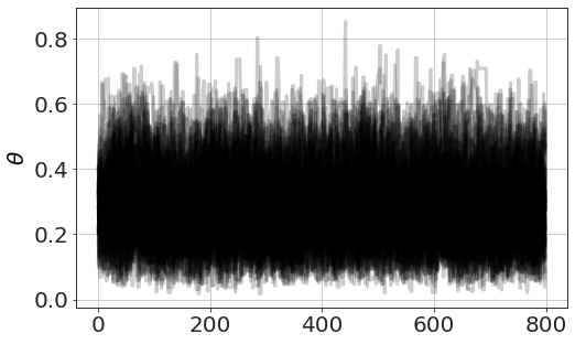
Now we run MCMC, plot the chains (so we can see it has converged) and look at distributions,
model.run_mcmc(800,repeat=3)
model.plot_chains()
Sampling Prior...
Done.
0.27 s
Running MCMC 1/3...
Done.
2.63 s
Running MCMC 2/3...
Done.
2.79 s
Running MCMC 3/3...
Done.
2.47 s
model.plot_distributions()
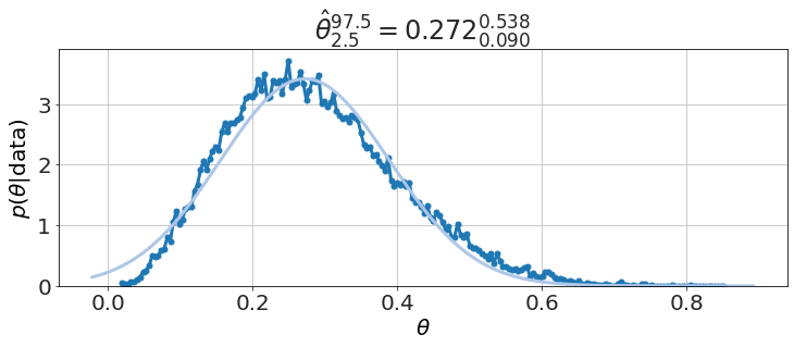
Is this evidence for a biased coin at, say, 95% level?
model.P("θ <0.5")
0.95485
yes, just as Lindley, 1976 presents.
The textbook only considers large sample proportions, with the definition \(f= h/N\). From the Beta distribution we get our estimate of the proportion
which matches the equations in the standard textbooks. Comparing to our case, with \(N=120\) we get good agreement,
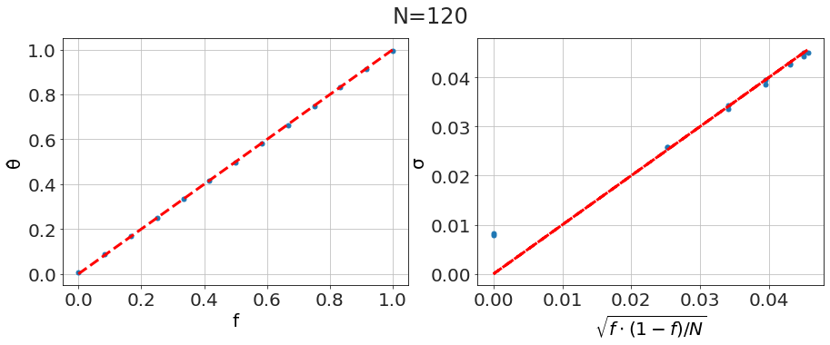
However, we start seeing differences where the textbook treatment isn't as informative as the methods we're using here. For small samples, say \(N=12\), we see that the textbook approximation breaks down -- especially near the \(f=0\) and \(f=1\) boundaries, sometimes overestimating our certainty and sometimes underestimating it.
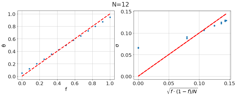
Notice, however, that in the current approach we didn't need to change anything to get more robust answers. Also notice that the current process for this problem is identical to the process for all of the other cases we've considered. So what we are presenting, compared to the textbook treatments, is a more unified approach which generalizes to small samples giving a more correct analysis for our data.
Gravitational Attraction
What would happen if two people out in space a few meters apart, abandoned by their spacecraft, decided to wait until gravity pulled them together? My initial thought was that …
A Simple Physics Problem Gets Messy
A physics problem from a practice AP test came to my attention, when my daughter was in AP physics this past spring. I went over her solutions when she did …

Skepticism and Dubious Medical Procedures
In my discussion with Jonathan McLatchie on the Still Unbelievable podcast, I said that there hasn’t been a verified miracle claim even since Hume’s essay on miracles. Here I look into the papers he references in response.
What problems are you interested in? How can I help?