Probability and the Independence of Testimony

Thu 23 February 2023 In #religion

In a previous post I examined a simple model of the interaction of testimony with scientific inquiry, and how it can affect the probabilities of the truth of miracle claims. In this post I examine a single result from Timothy and Lydia McGrews' article in The Blackwell Companion to Natural Theology entitled "Chapter 11 - The Argument from Miracles: A Cumulative Case for the Resurrection of Jesus of Nazareth". This paper is covered both in this YouTube episode, Bad Apologetics Ep 18 - Bayes Machine goes BRRRRRRRRR with Nathan Ormond, Kamil Gregor, and James Fodor, and summarized in text form on my blog starting here.

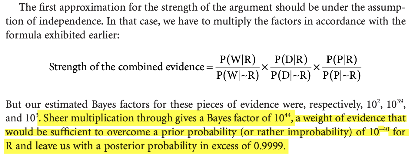
The result I want to look at is here:

Pasted image 20220713065658.png

The basic idea the McGrews have is that there are $N=15$ data points each with a Bayes factor of 1000, each completely independent from the others, leading to the product of probabilities yielding Bayes factor of around $1000^{15}=10^{45}$ (one of their Bayes factors is only 100 so they get $10^{44}$, but the idea is the same). I'll use $10^{45}$ in this post for mathematical simplicity below. We discuss in the video above how ridiculous $10^{44}$ is as a Bayes factor -- that there may not even be modern physical theories with Bayes factors that high. However, in this post, I want to take a direction that I haven't seen before but I think is enlightening.

TLDR: One can be supremely confident that all 15 sources are statistically independent, at probability of $p=0.9995$ (which is far higher than many scientific claims in published journals), and still not be able to justify the miracle claim due to the small uncertainty. This fact alone should disqualify the result the McGrews present.

Imperfect Information

One of the properties of all inference, particularly historical inference, is that there is some level of uncertainty. Do we know that, say, two claims in an ancient document are statistically independent? That's very hard to establish. The typical approach is to argue that the claims are textually independent and thus more likely to be statistically independent. This is a loose inference, because it is very easy for two texts to draw from the same oral tradition and thus not represent independent information. It's even hard in modern contexts to establish statistical independence between people making claims, even when you can interrogate the people and investigate the claims directly -- neither of which we can do for ancient texts.

So, that being said, it seems plausible that there is some degree of uncertainty in even establishing the independence of data sources. I'd like to explore how much uncertainty the McGrews calculation can tolerate and still maintain their argument. It is a sign of the strength of an argument if it can withstand some reasonable level of uncertainty.

Definitions

I use the same notation as I did in this post on testimony.

we have several data points, $D_1, D_2, \ldots, D_n$
we have the proposition, $M\equiv \text{a miracle occurred}$, for which we have a prior,
$$\begin{aligned} P(M) &\equiv m\\ P(\bar{M}) &\equiv 1-m\\ \end{aligned}$$
Note, that for miracle here you can substitute any extraordinary claim.

We're interested in $P(M|D_1, D_2, \ldots, D_n)$, but to establish a couple more definitions, let's look at the two-data case.

The two-data independent case

In the two data case we have

$$\begin{aligned} P(M|D_1, D_2) &= P(D_1|M)P(D_2|M,D_1)P(M)\\ P(\bar{M}|D_1, D_2) &= P(D_1|\bar{M})P(D_2|\bar{M},D_1)P(\bar{M})\\ \end{aligned} $$

We define the likelihood term for a single data point as,

$$\begin{aligned} P(D_1|M) &\equiv d\\ P(D_1|\bar{M}) &\equiv b \end{aligned}$$

The McGrews do not specify these probabilities numerically, but only specify their ratio, which is the single-point Bayes Factor they (arbitrarily) assume,

$$d/b=1000$$

They also assume independence of all the sources, which would imply,

$$\begin{aligned} P(D_2|M,D_1) &= P(D_2|M) \equiv d\\ P(D_2|\bar{M},D_1) &= P(D_2|\bar{M}) \equiv b \end{aligned}$$

The odds ratio then becomes,

$$ \begin{aligned} O &\equiv \frac{P(M|D_1, D_2)}{P(\bar{M}|D_1, D_2)} \\ &=\underbrace{\frac{P(D_1|M)\cdot P(D_2|M) }{P(D_1|\bar{M})\cdot P(D_2|\bar{M})}}_{\text{cumulative testimony}}\times \underbrace{\frac{P(M)}{P(\bar{M})}}_{\text{prior odds}} \\ &=\frac{d^2 \cdot m}{b^2\cdot (1-m)} \end{aligned} $$

The $n$-data independent case

Following the same procedure for $n$ points, we have,

$$ \begin{aligned} O &\equiv \frac{P(M|D_1, D_2, \ldots, D_n)}{P(\bar{M}|D_1, D_2, \ldots, D_n)} \\ &=\frac{P(D_1, D_2, \ldots, D_n|M)P(M)}{P(D_1, D_2, \ldots, D_n|\bar{M})P(\bar{M})} \\ &=\underbrace{\frac{P(D_1|M)\cdot P(D_2|M) \cdots P(D_n|M)}{P(D_1|\bar{M})\cdot P(D_2|\bar{M}) \cdots P(D_n|\bar{M})}}_{\text{cumulative testimony}}\times \underbrace{\frac{P(M)}{P(\bar{M})}}_{\text{prior odds}} \\ &= \frac{d^N}{b^N}\cdot \frac{P(M)}{P(\bar{M})} \end{aligned} $$

for the McGrews, $N=15$ and $d/b=1000$ and so they claim that the prior odds, $\frac{P(M)}{P(\bar{M})}$ needs to be less than $10^{-45}$ to overcome and they can't imagine that happening except for an overly skeptical person.

First look at dependence

Now what happens if the data are not independent or, if you prefer to avoid the double-negative, if the data are dependent? Then the probability of the second data point will be different, but how?

Imagine someone observes a fair coin that has been flipped and is lying on the table. They write down the result and leave the room. They then come back in, observe the coin and write the result. If during their absence,

someone flipped the coin again -- the second result will have the same probability as the first, and the result of the first flip will tell you nothing about the result of the second, $P(H_1)=1/2, P(H_2|H_1)=P(H_2)=1/2$ -- independent
no one touched the coin -- the second result is entirely determined by the first, $P(H_1)=1/2, P(H_2|H_1)=1$ -- dependent
someone turned the coin over on the table, changing heads to tails -- the second result is entirely determined by the first, $P(H_1)=1/2, P(H_2|H_1)=0$ -- dependent

Since we can have any possibility in between, we need to know the process of the dependence to determine at a minimum whether the value even goes up or down. In the case of testimony, it is far more likely for new testimony that is dependent on old testimony to give the same or similar information as the old. It would be odd indeed (even though the McGrews argue for this) for the new testimony to tend to be the opposite of the old. The consequences of this odd view is explored in the video and also in the summary here so I won't go into it in this post.

In the case of $D_2$ being completely dependent on $D_1$, it is the case that $D_2$ adds no new information. Or in other words, knowing $D_1$ it follows that $D_2$ is true necessarily,

$$\begin{aligned} P(D_2|M,D_1) &= 1\\ P(D_2|\bar{M},D_1) &= 1 \end{aligned}$$

In the $n$-data point case, this becomes,

$$ \begin{aligned} O &\equiv \frac{P(M|D_1, D_2, \ldots, D_n)}{P(\bar{M}|D_1, D_2, \ldots, D_n)} \\ &=\frac{P(D_1, D_2, \ldots, D_n|M)P(M)}{P(D_1, D_2, \ldots, D_n|\bar{M})P(\bar{M})} \\ &=\underbrace{\frac{P(D_1|M)\cdot P(D_2|M) \cdots P(D_n|M)}{P(D_1|\bar{M})\cdot P(D_2|\bar{M}) \cdots P(D_n|\bar{M})}}_{\text{cumulative testimony}}\times \underbrace{\frac{P(M)}{P(\bar{M})}}_{\text{prior odds}} \\ &=\underbrace{\frac{P(D_1|M)\cdot 1\cdots 1}{P(D_1|\bar{M})\cdot 1\cdots 1}}_{\text{cumulative testimony}}\times \underbrace{\frac{P(M)}{P(\bar{M})}}_{\text{prior odds}} \\ &= \frac{d}{b}\cdot \frac{m}{1-m} \end{aligned} $$

Using the McGrews numbers here, we get

$$ O= 1000 \cdot \frac{P(M)}{P(\bar{M})} $$

which means that the prior odds for a miracle need only be more then 1 in 1000 against to overcome this evidence -- not a very strong case for the miracle. Clearly dependent sources undermine the McGrews' case. But how much dependency is needed?

The first model

We'll start with the following simplified model of the uncertainty in the establishment of independence. For each data point after the first there is some probability that the data point is independent of the first. We'll call that value $\beta$. For intuition, note that

$\beta=1$ means we're certain the data point, $D_i$, is completely independent of the first, $D_1$
$\beta=0$ means we're certain the data point, $D_i$, is completely dependent on the first, $D_1$

Later we generalize this calculation to the case of partial dependency, but the conclusion is identical to this simpler model which is a little more intuitive.

For the 2-data point case we have,

$$ \begin{aligned} P(M|D_1,D_2)&=P(D_2|M,D_1)P(D_1|M)P(M) \\ &=(\beta\cdot d + (1-\beta)\cdot 1)\cdot d \cdot P(M) \end{aligned} $$

where the likelihood term for the second data point, $P(D_2|M,D_1)$ is broken up into two pieces -- a value of $d$ for the independent case with probability $\beta$ and a value of 1 for the dependent case with probability $1-\beta$. Generalizing this to the $n$-data point case,

$$ \begin{aligned} O &\equiv \frac{P(M|D_1, D_2, \ldots, D_n)}{P(\bar{M}|D_1, D_2, \ldots, D_n)} \\ &=\frac{(\beta d + (1-\beta))^{N-1}\cdot d}{(\beta b + (1-\beta))^{N-1}\cdot b}\cdot \frac{P(M)}{P(\bar{M})} \end{aligned} $$

Reproduce the McGrews' Result

To reproduce the result of the McGrews, we have the following:

$\beta=1$ : we're certain that the data are all independent
$d=10^{-3}$ and $b=10^{-6}$ giving an odds ratio for one data point $O=1000$.
$N=15$ (again, technically they have one point which has an odds ratio of 100 so their answer is $O=10^{44}$ whereas our answer here is $O=10^{45}$)

From the equation above we get

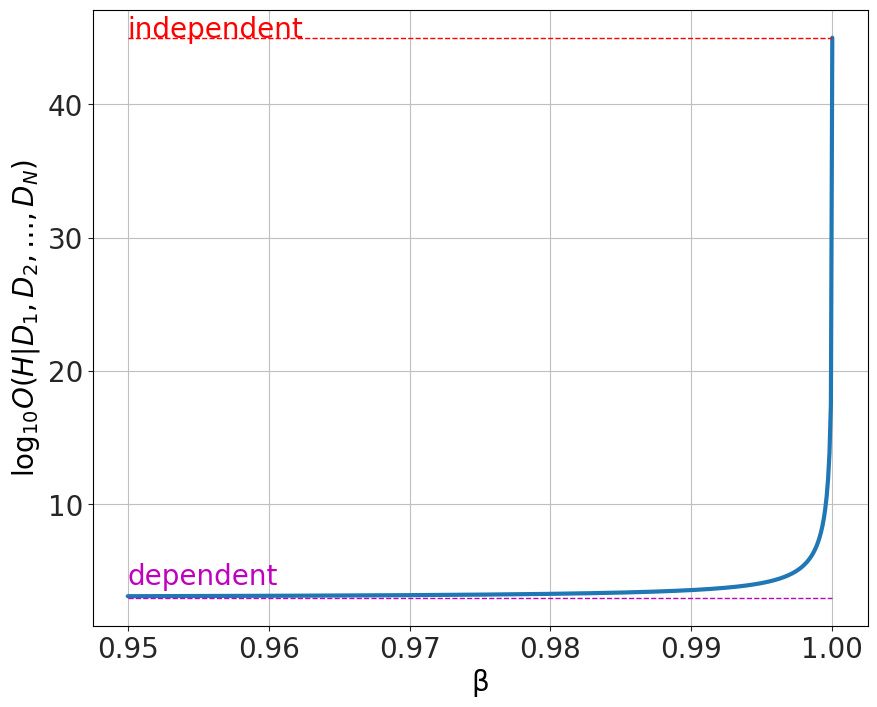
$$ \begin{aligned} O &\equiv \frac{P(M|D_1, D_2, \ldots, D_n)}{P(\bar{M}|D_1, D_2, \ldots, D_n)} \\ &=\frac{(1\cdot 10^{-3} + (1-1))^{15-1}\cdot 10^{-3}}{(1\cdot 10^{-6} + (1-1))^{N-1}\cdot 10^{-6} }\cdot \frac{P(M)}{P(\bar{M})}\\ &=10^{45}\cdot \frac{P(M)}{P(\bar{M})} \end{aligned} $$

How does the uncertainty affect the McGrews' Result?

The question here is how much uncertainty can this argument tolerate? In other words, how far can $\beta$ deviate from a value of 1 before the odds ratio comes down to a reasonable level?

An aside on a reasonable prior for the miracle

A very rough, maximum level for the prior for the Resurrection of Jesus can be obtained using the following logic. There are 8 billion people on the planet, perhaps twice that much in all of history, and (at least for the Christians) only one supported Resurrection. So that would mean, whether or not one believes in the Resurrection, the prior should be no larger than 1 in 10 billion. This I think is the maximum possible value of a prior I'd consider. It is comparable to the naive model the probability of the sun rising which I discuss elsewhere, without taking into account anything we have come to understand from science so is clearly an extremely conservative upper bound.

Back to the effect of $\beta$

We want to know where the first part of the odds ratio,

$$ \begin{aligned} \frac{(\beta d + (1-\beta))^{N-1}\cdot d}{(\beta b + (1-\beta))^{N-1}\cdot b} \end{aligned} $$

drops below $10^{10}$ so that the prior odds $\frac{P(M)}{P(\bar{M})}\sim 10^{-10}$ will overwhelm it and the argument fails. This point can be seen by observing a plot of the log base 10-odds ratio as a function of β and noting where the value dips below 10.

Pasted image 20230226182719.png This result surprised me. The tiniest deviation from the absolute certainty that all 15 sources are statistically independent brings the odds ratio down to the mundane. It drops below $10^{10}$ at around $\beta=0.9995$!

What this means is that one can be supremely confident that all 15 sources are statistically independent, at probability of $p=0.9995$ (which is far higher than many scientific claims in published journals), and still not be able to justify the miracle claim due to the small uncertainty. This fact alone should disqualify the result.

Partial dependency

One could criticize this result by saying that the choice isn't between perfectly independent and perfectly dependence, but that one can be partially dependent but mostly independent and that may be enough. TLDR on this section -- you get the same result as the previous solution.

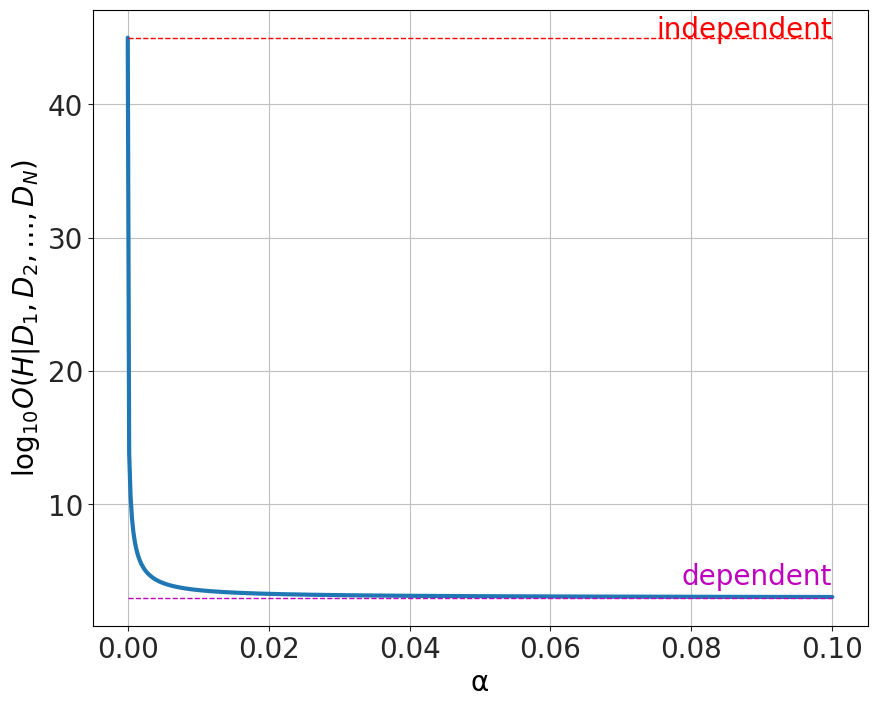
To handle this, we reparameterize the 2-data point case. Instead of the independent case $P(D_2|M,D_1)=d$ or the dependent case $P(D_2|M,D_1)=1$ we have a tunable version $P(D_2|M,D_1)=d+\alpha (1-d)$ where $\alpha$ measures how dependent each point is, from totally independent ($\alpha=0$) to totally dependent ($\alpha=1$). So each data point can be partially, but not totally, dependent. The $n$-data point generalization becomes

$$ \begin{aligned} O &=\frac{(d+\alpha (1-d))^{N-1}\cdot d}{(b + \alpha(1-b))^{N-1}\cdot b}\cdot \frac{P(M)}{P(\bar{M})} \end{aligned} $$

The question here is how far from the perfect independence can we have before things break. The result is the same as before, Pasted image 20230226184237.png

The tiniest deviation from independence results in the argument completely collapsing.

Conclusions

As stated before, what this means is that one can be supremely confident that all 15 sources are statistically independent, at probability of $p=0.9995$ (which is far higher than many scientific claims in published journals), and still not be able to justify the miracle claim due to the small uncertainty. This fact alone should disqualify the result.

Also, it speaks to the total naivety of the apologists calculations. They wrap their argument in seemingly technical and advanced Bayesian analyses, yet they don't seem to recognize that their argument comes down to assuming that testimony, evidence, and the scientific methods are identical to simple coin-flip experiments.

They ignore the effect of multiple models causing non-monotonic effects (see the high-low-nines deck example in Chapter 4 of Statistical Inference for Everyone which I also reference in a response to Jonathan McLatchie)
They ignore the impact that previous debunkings of claims affect the probability of the next claim given (see this post about testimony and the scientific process)
They ignore the possible uncertainty in the assumptions and data they are using, projecting an unwarranted confidence in the conclusions (this post)

So when I hear things like this from Jonathan McLatchie

"To this question, I would point out that (contrary to popular notions) it is not necessary for a hypothesis to be able to make high probability predictions in order for it to be well evidentially supported. Rather, it is only necessary that the pertinent data be rendered more probable given the hypothesis than it would be on its falsehood." (post here)

I remind myself that this is a totally simplistic way of approaching probability problems, especially in the case of things as messy as human testimony and ancient documents.