
Gravitational Attraction
What would happen if two people out in space a few meters apart, abandoned by their spacecraft, decided to wait until gravity pulled them together? My initial thought was that …

This is another in the series of "Statistics 101" examples solved with MCMC. Others in the series:
In all of these posts I'm going to use a python library I make for my science-programming class, stored on github, and the emcee library. Install like:
pip install "git+git://github.com/bblais/sci378" --upgrade
pip install emcee
In this example, like another one in the series, there is some true value, we call \(x_o\). The \(N\) data points we have, \(\{x_i\}\), consist of that true value drawn from a particular distribution, in this case the Cauchy distribution:

This distribution has a number of applications, many of which occur in cases of circular geometry. I was introduced to it with the so-called lighthouse problem and E T Jaynes's excellent Confidence Intervals vs Bayesian Intervals paper.
Although this distribution has a single-peak with a central value, \(x_o\), and looks vaguely Gaussian, it has many mathematical properties which make it much different. For example, it has an undefined mean and variance, and thus doesn't satisfy the conditions for the central limit theorem. As such it is never covered in introductory statistics classes. However, with the computational approach described here, it is no harder to work with the Cauchy than the Normal.
In E T Jaynes's example, the data consist simply of two data points: \(\{x_i\} = \{3,5\}\). Remarkably, frequentist methods can't address this problem. The likelihood is set in the same way as previous posts:
def lnlike(data,x_o,γ):
    x=data
    return logcauchypdf(x,x_o,γ)

data=array([3.,5])
model=MCMCModel(data,lnlike,
                x_o=Uniform(-50,50),
                γ=Jeffreys()
                )
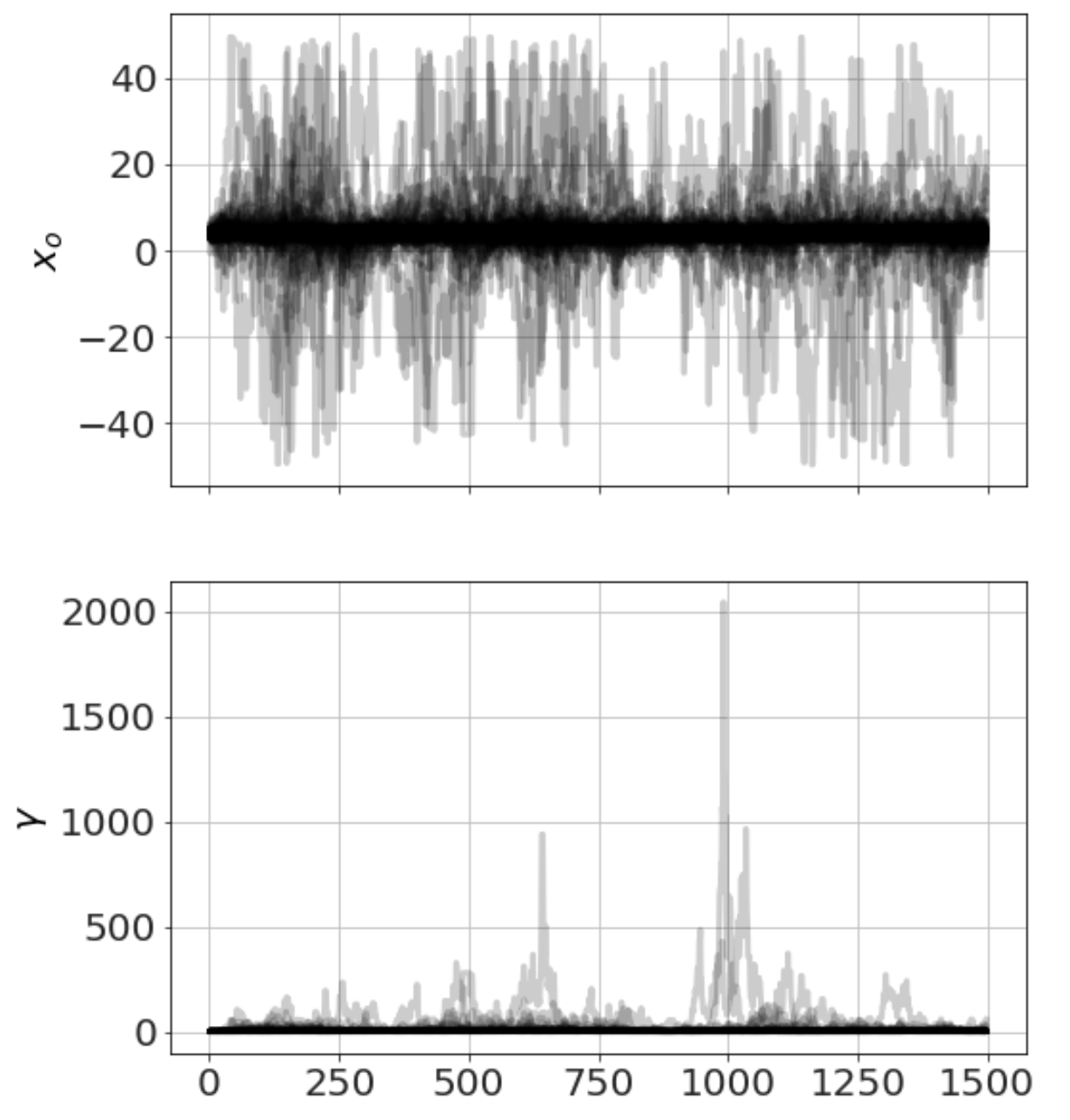
Now we run MCMC, plot the chains (so we can see it has converged) and look at distributions,
model.run_mcmc(1500,repeat=3)
model.plot_chains()
Sampling Prior...
Done.
0.43 s
Running MCMC 1/3...
Done.
3.74 s
Running MCMC 2/3...
Done.
3.61 s
Running MCMC 3/3...
Done.
3.66 s
model.plot_distributions()
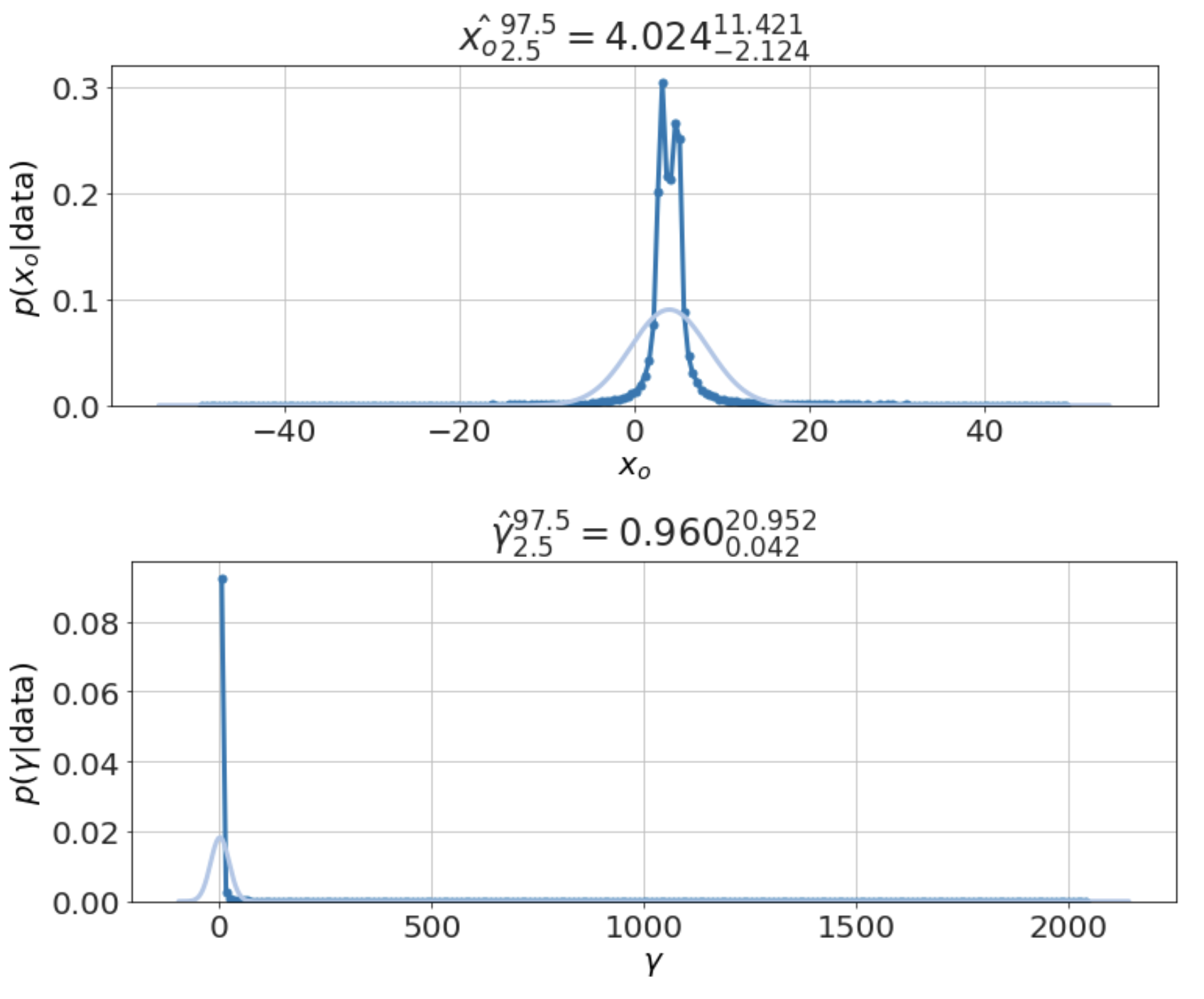
Although the Cauchy has no defined mean value, one can show that the median of the data is a best estimate for the central value, \(x_o\) -- although that doesn't give the uncertainties. Thus, the estimate we find above, \(x_o \sim 4\), matches what we intuit to be the correct answer.
The point here, however, is that the same Bayesian methods for finding the best estimates and the uncertainties works for this case like all the others -- with very little extra work -- whereas traditional methods fail. It is telling that statistics textbooks uniformly ignore this entire distribution as far as I can tell just to avoid the problems with it. The Bayesian approach, in contrast, provides a uniform procedure to address all such problems and that procedure consistently produces useful results.
Gravitational Attraction
What would happen if two people out in space a few meters apart, abandoned by their spacecraft, decided to wait until gravity pulled them together? My initial thought was that …

A Simple Physics Problem Gets Messy
A physics problem from a practice AP test came to my attention, when my daughter was in AP physics this past spring. I went over her solutions when she did …

Skepticism and Dubious Medical Procedures
In my discussion with Jonathan McLatchie on the Still Unbelievable podcast, I said that there hasn’t been a verified miracle claim even since Hume’s essay on miracles. Here I look into the papers he references in response.
What problems are you interested in? How can I help?